Quantitative eDNA Metabarcoding: A Spike-In DNA Framework for Robust Biomonitoring and Biomedical Application

Abstract

Quantitative environmental DNA (eDNA) metabarcoding is revolutionizing biodiversity monitoring and ecological assessment by moving beyond simple presence-absence data to deliver quantitative species abundance estimates. This article explores the integration of internal spike-in DNAs as a critical methodological advancement that corrects for technical biases in amplification and sequencing, thereby transforming metabarcoding into a truly quantitative tool. We provide a comprehensive framework covering the foundational principles of the technique, detailed methodological protocols for spike-in implementation, strategies for troubleshooting and optimizing performance, and rigorous validation against traditional survey methods. Tailored for researchers and drug development professionals, this review highlights the transformative potential of quantitative eDNA metabarcoding for applications ranging from ecosystem health assessment to monitoring environmental impacts of pharmaceuticals.

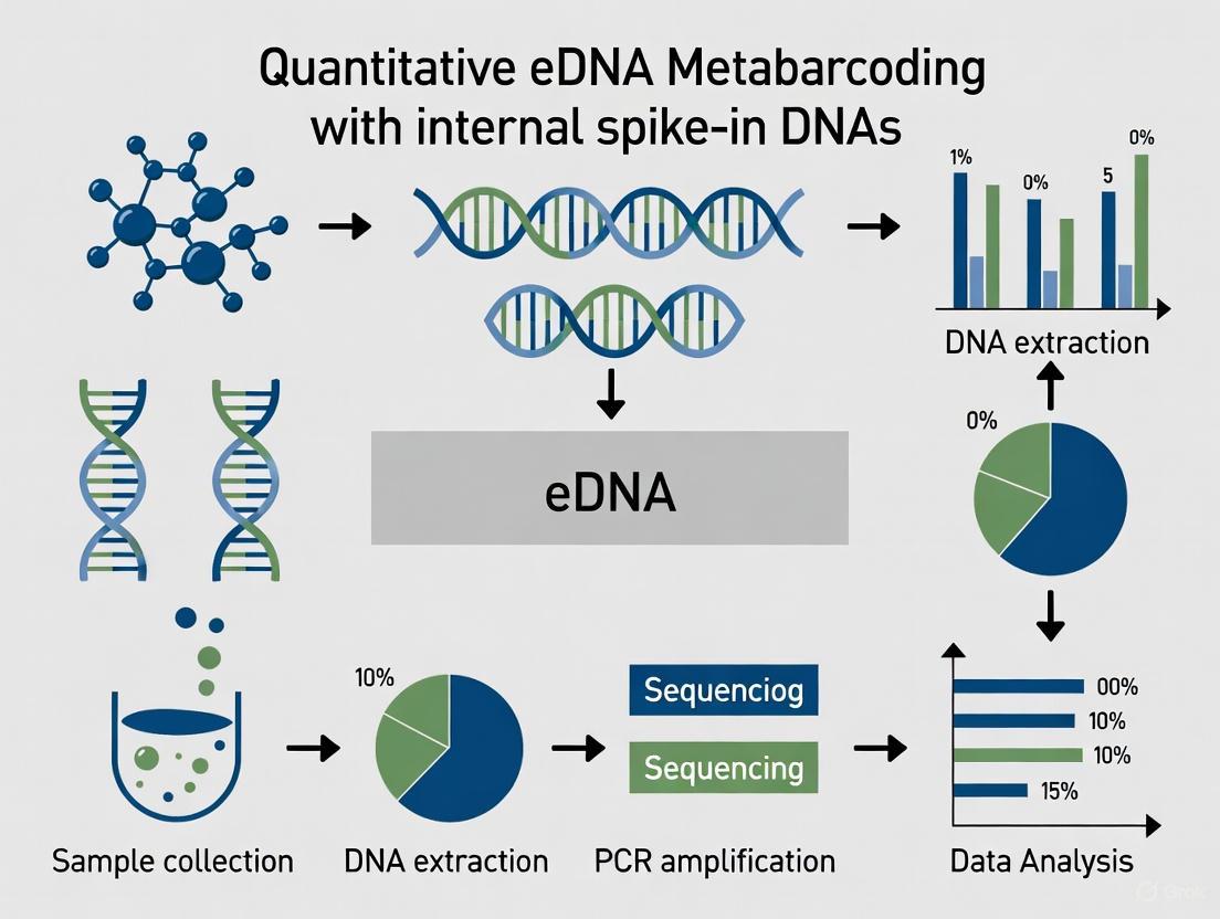
The Principles and Promise of Quantitative eDNA Metabarcoding

The field of environmental DNA (eDNA) analysis has rapidly evolved, transitioning from simple presence-absence detection to sophisticated quantitative applications. This shift is particularly crucial in biomonitoring, where understanding species abundance and biomass is essential for effective conservation and ecosystem management. Traditional presence-absence data provides limited ecological insights, whereas quantitative approaches enable researchers to track population trends, assess ecosystem health, and evaluate human impacts with unprecedented precision. The integration of internal spike-in DNAs represents a transformative advancement, allowing for correction of technical variations throughout the molecular workflow and generating truly quantitative data. This protocol details comprehensive methodologies for implementing quantitative eDNA metabarcoding approaches, focusing on experimental design, procedural standardization, and data normalization techniques that move beyond basic detection to provide robust abundance metrics [1].

Experimental Protocols for Quantitative eDNA Analysis

Sample Collection and Filtration Protocol

Materials Required:

• Sterile sampling bottles (1-3L capacity)
• Filtration apparatus with pump system
• Filter membranes (1µm and 5µm pore sizes)
• Sterile forceps and gloves
• Sample preservation buffer (e.g., Longmire's buffer, ethanol)
• Cold storage containers for transport

Procedure:

• Collect water samples in sterile containers, avoiding surface disturbance. Take biological replicates (typically 3-5) from each sampling location to account for natural spatial heterogeneity [1].
• Pre-measure water volumes (1L and 3L comparisons) for consistent processing across samples.
• Assemble filtration apparatus using appropriate pore size filters (1µm for microbial communities; 5µm for metazoan/vertebrate targets) [1].
• Filter water samples through designated filter membranes using a peristaltic pump or vacuum system.
• Using sterile forceps, carefully transfer filters to preservation tubes containing appropriate buffer.
• Store samples immediately at -20°C or in liquid nitrogen for transport to laboratory.
• Document filtration time, volume filtered, filter pore size, and preservation method for each sample.

Technical Considerations: Larger pore size filters (5µm) and larger water volumes (3L) maximize the ratio of amplifiable target DNA to total DNA for vertebrate species without compromising absolute detection. For microbial targets, smaller pore sizes (0.22-0.45µm) remain preferable due to smaller particle sizes and higher abundance of microbial DNA in the environment [1].

DNA Extraction and Internal Spike-In Implementation

Materials Required:

• DNA extraction kits (e.g., DNeasy PowerWater Kit, phenol-chloroform reagents)
• Synthetic internal spike-in DNA (non-competitive, species-specific)
• Quantitative PCR (qPCR) instrumentation and reagents
• Spectrophotometer or fluorometer for DNA quantification
• Microcentrifuges and thermal cyclers

Procedure:

• Spike-In DNA Preparation:
  • Design synthetic DNA sequences with similar length and GC content to target DNA but containing unique primer binding sites.
  • Quantify spike-in DNA accurately using fluorometric methods.
  • Create a dilution series to establish standard curves for absolute quantification.

• DNA Extraction with Spike-Ins:

  • Add known quantities of spike-in DNA to each sample immediately before extraction.
  • Extract DNA using standardized protocols (commercial kits or phenol-chloroform methods).
  • For vertebrate targets, phenol-chloroform extraction may maximize total DNA recovery but can co-extract inhibitors [1].
  • Evaluate extraction efficiency by comparing expected vs. recovered spike-in concentrations.

• Quality Assessment:

  • Quantify total DNA yield using spectrophotometric methods.
  • Assess DNA quality via gel electrophoresis or bioanalyzer.
  • Aliquot extracted DNA for downstream applications and store at -80°C.

Technical Considerations: Maximizing total DNA yield during extraction does not always increase target detection, as it may concentrate inhibitors and co-extracted off-target DNA. The optimal extraction method should maximize the target-to-total DNA ratio rather than total DNA alone [1].

Data Presentation and Analysis

Quantitative Comparison of Methodological Parameters

Table 1: Impact of Filtration Parameters on Target DNA Recovery

Parameter	Condition	Target DNA Yield	Total DNA Yield	Target:Total Ratio	Inhibition Risk
Filter Pore Size	1µm	Low	High	Low	Moderate
	5µm	High	Moderate	High	Low
Water Volume	1L	Low	Low	Moderate	Low
	3L	High	High	High	Moderate-High
Filter Material	Cellulose nitrate	Moderate	Moderate	Moderate	Low
	Glass fiber	High	High	High	Moderate

Table 2: Comparison of DNA Extraction Methods for Vertebrate eDNA

Extraction Method	Total DNA Yield	Target DNA Recovery	Inhibitor Co-extraction	Processing Time	Cost
Phenol-Chloroform	High	Variable	High	Long	Low
Silica Membrane Kit	Moderate	Consistent	Low	Short	Moderate
Magnetic Bead Kit	Moderate-High	Consistent	Very Low	Short	High

Statistical Modeling for Data Integration

The following statistical approach allows inclusion of data from samples collected and processed using different protocols:

• Linear Model Framework:

  • Develop a normalization model using spike-in recovery rates to correct for technical variations.
  • Incorporate protocol-specific correction factors for filter type, volume, and extraction method.
  • Account for biological variability through replicate sampling and random effects in mixed models.

• Data Integration Equation:

• Variance Partitioning:

  • Separate technical variance (extraction, amplification) from biological variance (spatial heterogeneity).
  • Use coefficient of variation (CV) calculations to assess method precision [1].

Visualization of Experimental Workflows

Quantitative eDNA Metabarcoding Workflow

Internal Spike-In Normalization Logic

The Scientist's Toolkit: Essential Research Reagents

Table 3: Research Reagent Solutions for Quantitative eDNA Studies

Reagent/Material	Function	Application Notes
Synthetic Spike-In DNA	Internal standard for quantification	Designed with unique barcodes; non-competitive with target species; added pre-extraction
Filter Membranes (5µm)	Particle capture for vertebrate eDNA	Optimized for metazoan DNA recovery; reduces microbial DNA background
Inhibition Resistance PCR Mix	Enhanced amplification efficiency	Critical for complex environmental samples; reduces false negatives
DNA Preservation Buffer	Biomolecule stabilization	Long-term integrity of eDNA; compatible with downstream applications
Quantitative PCR Reagents	Absolute quantification	Standard curves for spike-in and target DNA; high precision required
Metabarcoding Primers	Taxon-specific amplification	Designed for complementary regions; validated for quantitative recovery
Bioinformatic Pipelines	Data processing and normalization	Custom scripts for spike-in normalized quantification; open-source options available
2-Methylbutyrylglycine-d9	2-Methylbutyrylglycine-d9 Deuterated Standard	2-Methylbutyrylglycine-d9 is a deuterium-labeled internal standard for RUO quantification of 2-MBG in metabolic disorder research. For Research Use Only.
1,7-Bis(4-hydroxyphenyl)hept-1-en-3-one	1,7-Bis(4-hydroxyphenyl)hept-1-en-3-one, MF:C19H20O3, MW:296.4 g/mol	Chemical Reagent

The implementation of quantitative eDNA metabarcoding with internal spike-in DNAs represents a paradigm shift in biomonitoring capabilities. By moving beyond simple presence-absence data, researchers can now generate abundance metrics that provide deeper ecological insights and more robust environmental assessments. The protocols outlined herein emphasize methodological standardization while acknowledging the need for flexibility in protocol selection based on specific research questions and target organisms. Future developments in synthetic spike-in design, multi-species quantification approaches, and integrated bioinformatic pipelines will further enhance the precision and applicability of quantitative eDNA methods. As the field continues to evolve, the framework presented here provides a foundation for generating comparable, reproducible quantitative data across studies and ecosystems, ultimately supporting more effective conservation and management decisions.

Internal spike-in DNAs are known quantities of exogenous or synthetic DNA sequences added to biological samples to serve as an internal reference for quantitative normalization. In quantitative environmental DNA (eDNA) metabarcoding, they function as a critical quality control tool, enabling researchers to calibrate measurements, account for technical biases introduced during sample processing, and transition from relative to absolute abundance estimates. This protocol outlines the fundamental principles, implementation workflows, and key applications of spike-in DNAs, providing a framework for their use in robust and reproducible eDNA-based biomonitoring.

In molecular biology, particularly in sequencing-based assays, the accurate quantification of target molecules is often hampered by numerous technical variabilities. Internal spike-in DNAs are known quantities of molecules—such as oligonucleotide sequences—added to a biological sample to act as an internal reference for the quantitative estimation of the molecule of interest across samples and batches [2]. Their primary role is to correct for technical and biological biases introduced during sample processing, including DNA extraction, library preparation, handling, and sequencing [2].

Within the specific context of quantitative eDNA metabarcoding, the use of spike-in controls has emerged as a powerful strategy to overcome the limitations of standard read-count normalization. In metabarcoding, the total DNA signal can vary significantly between samples due to biological reasons (e.g., differences in total biomass) or technical artifacts. Normalizing by total read count can introduce severe biases and lead to misleading biological interpretations [3]. Spike-in controls, added at the very beginning of the workflow, experience the same technical processes as the endogenous eDNA. The discrepancy between the known amount of spike-in added and the finally measured amount provides a sample-specific scaling factor that can be applied to the native eDNA data, thereby improving the accuracy of inter-sample comparisons and enabling absolute quantification [4].

The Working Principle and Normalization Strategy

The core principle of spike-in DNAs is based on their use as an internal standard. A precise, known quantity of spike-in DNA is added to each sample during the initial processing steps. Following sequencing and bioinformatic analysis, the recovery rate of the spike-in sequences is calculated. This recovery rate directly reflects the cumulative technical efficiency and bias of the entire workflow for that specific sample.

The following workflow diagram illustrates the typical lifecycle of a spike-in control within a sample, from addition to final data normalization:

The normalization process typically involves deriving a sample-specific scaling factor. A common approach involves determining the ratio between the observed spike-in read counts and the expected counts. For instance, if a sample yields fewer spike-in reads than expected, its endogenous gene counts are scaled upwards, under the assumption that the lower spike-in recovery reflects a global technical loss for that sample [2]. More sophisticated methods may use regression analysis or factor analysis across multiple spike-ins added at various concentrations to model the relationship between input amount and sequencing output for a more robust estimate of technical bias [2].

Types of Spike-Ins and Research Reagent Solutions

The choice of spike-in type depends on the experimental goals, the required precision, and practical considerations regarding availability and cost. The table below summarizes the three main types of DNA spike-ins used in metabarcoding studies:

Table 1: Comparison of Primary DNA Spike-In Types for Metabarcoding

Spike-In Type	Description	Advantages	Limitations
Biological Spike-Ins [4]	Whole organisms or intact cells from a different species (e.g., Drosophila cells added to human samples).	Contains a diverse, natural set of target epitopes; easy to integrate into workflows.	Input DNA amount is difficult to control and quantify precisely; long-term supply can be challenging.
DNA Spike-Ins [4]	Pre-amplified marker DNA from a non-target organism.	Allows for more precise measurement of input material than biological spike-ins.	The original biological source is finite; potential for degradation; difficult to recreate if lost.
Synthetic Spike-Ins [4]	Artificial DNA molecules designed in silico and commercially synthesized.	Can be precisely quantified; sequence is customizable; can be resynthesized infinitely; easily distinguished from sample DNA.	Requires careful design and synthesis; may not perfectly mimic all properties of natural DNA.

The selection of the appropriate spike-in is a critical decision. Synthetic spike-ins are increasingly recommended for long-term monitoring projects due to their infinite reproducibility and precise quantifiability [4].

Research Reagent Solutions

The successful implementation of a spike-in protocol relies on key reagents and materials. The following table details essential components and their functions.

Table 2: Key Research Reagents for Spike-In Experiments

Reagent / Material	Function / Description	Example Application
Synthetic DNA Fragments [4]	Custom-designed, artificially generated DNA sequences that serve as the spike-in standard.	Designed to be amplified by the same universal primers as the target eDNA but be unique enough for bioinformatic separation.
Universal Primers [5]	Primer sets that amplify a standardized, taxonomically informative gene region from both the sample eDNA and the spike-in.	The MiFish-U primer set is a universal primer for fish eDNA metabarcoding [5].
High-Fidelity DNA Polymerase [3]	PCR enzyme with proofreading activity to minimize amplification errors during library preparation.	Critical for accurate amplification of both spike-in and sample sequences in quantitative assays.
Quantitative Standard [3]	A pre-quantified sample of the spike-in DNA used to create a dilution series for a standard curve.	Used in qPCR to absolutely quantify the spike-in DNA before it is added to experimental samples.
External RNA Controls Consortium (ERCC) Spike-Ins [2]	A well-known set of synthetic spike-in standards developed for RNA-seq that exemplifies the principle for DNA-based assays.	Serves as a model for designing and implementing complex spike-in mixtures for DNA metabarcoding.

Quantitative Evidence and Validation

The utility of spike-in normalization is not merely theoretical; it is backed by empirical evidence demonstrating its superiority over conventional normalization methods. The following table summarizes key quantitative findings from selected studies that validate the spike-in approach:

Table 3: Quantitative Evidence Supporting Spike-In Normalization

Study Context	Spike-In Method	Key Quantitative Finding	Implication
Fish Community Monitoring [5]	qMiSeq (using internal standard DNAs)	Significant positive relationships were found between eDNA concentrations quantified by qMiSeq and both abundance (R² values provided) and biomass of captured fish across 21 river sites.	Demonstrated that spike-in normalized eDNA metabarcoding is a suitable tool for quantitative monitoring of fish communities.
Chromatin Immunoprecipitation (ChIP) [6]	ChIP-Rx (using exogenous chromatin)	In a titration of H3K79me2 levels over a 10-fold range, spike-in normalization correctly quantified enrichment across the signal intensity range, whereas read-depth normalization failed.	Showed spike-in normalization provides accurate quantification across a wide dynamic range where standard methods fail.
R-loop Mapping (DRIP-seq) [3]	Synthetic RNA-DNA hybrids & Drosophila cellular spike-ins	After global transcription inhibition, read-count normalization created an artifactual increase in signal at the 3' ends of long genes. Spike-in normalization corrected this, showing no change, which was validated by DRIP-qPCR.	Highlighted that without spike-in normalization, global changes in total target content can lead to severe misinterpretations.

Detailed Experimental Protocols

Protocol A: Implementing Synthetic Spike-Ins for eDNA Metabarcoding

This protocol is adapted from recommendations for insect metabarcoding using the COI gene, a common practice that can be adapted for other target taxa [4].

• Spike-in Design: Design one or more synthetic DNA sequences in silico that:
  • Contain the binding sites for your universal metabarcoding primers (e.g., MiFish-U for fish [5]).
  • Are highly divergent from any natural sequence in public databases to prevent misidentification. A BLAST search is essential.
  • Are of a length similar to the expected amplicon from the native eDNA.
• Spike-in Synthesis: Commission the synthesis and cloning of the designed sequence(s) from a commercial vendor. Receive the product typically as a plasmid in a bacterial stock.
• Spike-in Quantification:
  • Isolate the plasmid and linearize it.
  • Quantify the DNA concentration accurately using a fluorometer. Calculate the exact copy number/µL based on the molecular weight.
  • Serially dilute the stock to create a working solution of known concentration (e.g., 10^8 copies/µL).
• Spike-in Addition: Add a fixed, small volume (e.g., 2 µL) of the working solution to each eDNA sample extract immediately after extraction and before any amplification steps. The amount added should be within the same order of magnitude as the expected target eDNA to be quantitatively meaningful. Vortex thoroughly.
• Metabarcoding PCR and Sequencing: Proceed with standard library preparation using your universal primers. The spike-in sequences will be co-amplified with the native eDNA.
• Bioinformatic Separation:
  • Process the raw sequencing data through your standard pipeline (e.g., quality filtering, denoising).
  • Using a reference file of the synthetic spike-in sequence(s), separate the spike-in-derived Amplicon Sequence Variants (ASVs) from the native eDNA ASVs.
• Normalization Calculation and Application:
  • For each sample, calculate the normalization factor (NF). A simple method is: NF_sample = (Total Spike-in Reads in Sample) / (Average Total Spike-in Reads across all Samples)
  • Divide the read count of each native eDNA ASV in a sample by the NF for that sample to obtain the normalized abundance.

Protocol B: Using a Cellular Spike-In for DRIP-Seq

This protocol details the use of Drosophila melanogaster cells as a spike-in for DNA-RNA Immunoprecipitation Sequencing (DRIP-seq), a method applicable to other chromatin studies [3].

• Spike-in Cell Culture: Maintain a culture of Drosophila melanogaster S2 cells under standard conditions.
• Sample and Spike-in Mixing:
  • Harvest the human (or target) cells and the Drosophila cells by centrifugation.
  • For each experimental sample, mix a fixed number of Drosophila cells (e.g., 1 x 10^6 cells) with a fixed number of human cells (e.g., 10 x 10^6 cells). The ratio should be consistent across all samples.
  • Co-pellet the mixed cells.
• Chromatin Preparation and DRIP: Isolate chromatin from the mixed cell pellet according to your standard DRIP or ChIP protocol [3]. The key is that the Drosophila chromatin is subjected to the exact same conditions (lysis, sonication/shearing, immunoprecipitation with the S9.6 antibody, etc.) as the human chromatin.
• Library Preparation and Sequencing: Construct sequencing libraries from the immunoprecipitated DNA and sequence on an appropriate platform.
• Bioinformatic Analysis and Normalization:
  • Align the sequencing reads to a combined reference genome (e.g., human + Drosophila).
  • Separate the reads aligning to the Drosophila genome.
  • Identify a set of high-confidence peaks from the Drosophila signal.
  • Sum the reads mapping within these Drosophila peaks for each sample.
  • Calculate a normalization factor for each sample based on the total Drosophila reads (or peak reads), for example, using the median of ratios method [3]. Apply this factor to the reads mapping to the human genome.

Internal spike-in DNAs are no longer a niche tool but a fundamental component for rigorous quantitative eDNA metabarcoding and other sequencing applications. By providing an internal reference that travels with the sample through the entire workflow, they empower researchers to distinguish technical noise from biological signal, compare data across different batches and studies, and move beyond simple presence-absence data towards meaningful absolute abundance estimates. The adoption of standardized spike-in protocols, particularly using sustainable synthetic standards, is a critical step towards achieving comparability and standardization in global biomonitoring efforts [4]. As the field advances, the integration of spike-ins will be paramount for generating the high-fidelity, quantitative data necessary to understand and manage ecosystems effectively.

The simultaneous conservation of species richness and evenness is paramount for effectively reducing biodiversity loss and maintaining ecosystem health [7]. Traditional methods for biomonitoring, such as direct capture and visual census, provide valuable data but are often constrained by the requirement for significant effort, time, and taxonomic expertise [7]. Furthermore, these methods can be invasive, potentially damaging fragile populations of endangered species and their habitats [7]. Environmental DNA (eDNA) analysis has emerged over the past decade as a powerful, non-invasive alternative for detecting organisms through the cellular materials they shed into their environment [7].

Environmental DNA analysis for macroorganisms primarily utilizes two technical methods: species-specific detection and DNA metabarcoding. The species-specific approach, often using quantitative PCR (qPCR), is a established method for absolute quantification but is limited in scope. The development of species-specific assays is time-consuming, costly, and requires prior knowledge of the species present in a study area, making it unsuitable for the simultaneous quantitative assessment of multiple, unexpected species in a community [7]. In contrast, eDNA metabarcoding, which uses universal primers and high-throughput sequencing, allows for the comprehensive identification of community composition across multiple taxa [7] [8]. However, a significant challenge has been that the sequence read counts generated are not directly quantitative. These read counts can be skewed by PCR amplification biases, primer mismatches, and library preparation artifacts, preventing them from reliably representing the true biomass or abundance of species in the environment [7] [8]. The qMiSeq approach was developed to bridge this critical gap, transforming metabarcoding from a primarily qualitative tool into one capable of absolute quantification [7].

The qMiSeq Approach: Principle and Workflow

The quantitative MiSeq sequencing (qMiSeq) approach is a novel method that enables the conversion of sequence read numbers into absolute DNA copy numbers [7]. Its core innovation lies in the use of internal standard DNAs that are spiked into each sample at known concentrations before PCR amplification. This allows for the creation of a sample-specific standard curve, which accounts for technical variations that occur during the analytical process.

The principle of qMiSeq is based on generating a linear regression between the known copy numbers of the internal standards and the sequence reads they generate in each sample [7]. The resulting regression coefficient is then used to convert the sequence reads of detected native taxa in that same sample into estimated DNA copy numbers. This controls for sample-specific effects like PCR inhibition and library preparation bias, which are major hurdles for quantitative metabarcoding [7]. A standard curve is essential in quantitative PCR methods to determine unknown target concentrations [9], and qMiSeq adapts this robust principle for a high-throughput sequencing context.

The following workflow diagram outlines the key procedural steps in a qMiSeq experiment, from sample collection to data interpretation.

Key Advantages of the Internal Standard Method

The use of internal standards differentiates qMiSeq from conventional metabarcoding and provides its quantitative power. The internal controls allow for estimating the expected initial copy number of the target by accounting for the variable efficiency of the PCR amplification and other preparatory steps [10]. The internal standard method is designed to yield approximately unbiased answers, provided that the key assumptions of the technique are met, such as equivalent amplification efficiency between standards and target molecules [10]. This method provides a means to control for the exponential nature of PCR, where small variations in amplification efficiency can lead to large differences in the final product yield [11].

Experimental Validation and Key Quantitative Data

The performance of the qMiSeq approach as a quantitative monitoring tool has been rigorously validated through controlled studies. One such study compared eDNA concentrations quantified by qMiSeq with the results of traditional capture surveys using an electrical shocker across 21 sites in four rivers in Japan [7]. The findings demonstrated a significant positive relationship between the eDNA concentrations of each species quantified by qMiSeq and both the abundance and biomass of each captured taxon at the study sites [7].

The table below summarizes the key quantitative relationships observed in this validation study.

Table 1: Summary of Validation Results Comparing qMiSeq with Capture Surveys

Comparison Metric	Relationship Observed	Statistical Significance	Context
eDNA conc. vs. Abundance/Biomass	Significant positive relationship	P-value < 0.05	Multi-species data within sites [7]
eDNA conc. vs. Abundance/Biomass	Significant positive relationship for 7 out of 11 taxa	P-value < 0.05	Within individual taxa across multiple sites [7]
Species Richness	qMiSeq consistently detected more species than capture surveys	N/A	At 16 out of 21 sites, no false negatives occurred [7]
qMiSeq vs. qPCR	Significant positive relationship for 3 tested taxa	P < 0.001, R² = 0.81-0.99	Validation against an established quantitative method [7]

This validation confirms that the qMiSeq approach can produce biologically meaningful quantitative data. The high correlation with both capture survey data and independent qPCR assays underscores its reliability and potential to replace or supplement more invasive and labor-intensive methods.

Detailed qMiSeq Protocol

This section provides a detailed step-by-step protocol for implementing the qMiSeq approach for the absolute quantification of fish communities from water samples.

Sample Collection and Filtration

• Water Collection: Collect water samples in sterile containers from the target environment (e.g., river, lake, marine water). The volume collected should be standardized; 1-2 liters is common for freshwater systems. Field blanks (e.g., ultra-pure water transported to the field) should be included to control for contamination.
• Filtration: Filter water samples through sterile membrane filters (e.g., mixed cellulose ester, glass fiber) with a pore size of 0.2 to 1.0 µm to capture eDNA particles. The choice of filter material and pore size may be optimized for the specific environmental matrix and biomass load.
• Preservation: Preserve the filters immediately after filtration. They can be stored frozen at -20°C or in a preservation buffer (e.g., Longmire's buffer, ethanol) to prevent DNA degradation.

DNA Extraction and Internal Standard Addition

• Extraction: Extract DNA from the filters using a commercial DNA extraction kit suitable for environmental filters. Follow the manufacturer's protocol, but include negative extraction controls (reagents only) to monitor for contamination.
• Internal Standard Spike-In: After extraction, spike a known quantity of synthetic internal standard DNAs into each sample extract. These standards should be non-competitive, artificial sequences that are amplified by the same universal primers but are distinguishable bioinformatically. A dilution series of at least 3-5 different concentrations is recommended to construct a robust standard curve [7]. The exact copy number of each standard must be known.

Library Preparation and Sequencing

• Amplification: Perform a PCR amplification on the sample-spike mix using universal primers targeting the taxonomic group of interest (e.g., the MiFish-U primer set for fish [7]). The PCR conditions (annealing temperature, cycle number) should be optimized to minimize bias and maximize specificity.
• Library Construction: Prepare sequencing libraries from the amplified products according to the requirements of the chosen high-throughput sequencing platform (e.g., Illumina MiSeq/iSeq). This typically involves a second, limited-cycle PCR to add platform-specific adapter sequences and sample-indexing barcodes to allow for multiplexing.
• Sequencing: Pool the indexed libraries in equimolar concentrations and sequence on an appropriate platform (e.g., iSeq for smaller studies, MiSeq for larger ones). The sequencing run should generate a sufficient number of reads to cover all samples and expected diversity without being saturated.

Data Analysis and Absolute Quantification

• Bioinformatics: Process the raw sequence data through a standard metabarcoding pipeline. This includes demultiplexing, quality filtering (e.g., using QIIME2 or DADA2), merging paired-end reads, and clustering sequences into Operational Taxonomic Units (OTUs) or Amplicon Sequence Variants (ASVs). Taxonomic assignment is performed by comparing these units to a reference database.
• Standard Curve Generation: For each sample, plot the known copy numbers of the internal standards against their obtained sequence reads. Perform a linear regression analysis to derive the sample-specific coefficient (slope) for converting reads to copies [7].
• Absolute Quantification: Apply the sample-specific regression coefficient to the sequence read counts of all biologically relevant taxa detected in that sample. This calculation yields the estimated absolute DNA copy number for each taxon in the original sample. The conceptual relationship between the internal standards and the quantitative result is illustrated below.

The Scientist's Toolkit: Essential Reagents and Materials

Successful implementation of the qMiSeq approach requires careful selection of reagents and materials. The following table details the key components and their functions.

Table 2: Essential Research Reagent Solutions for the qMiSeq Approach

Item	Function / Role	Key Considerations
Universal Primers (e.g., MiFish-U)	To amplify a standardized DNA barcode region from all target taxa (e.g., fish) in the community.	Must be broadly conserved across the taxonomic group while providing sufficient taxonomic resolution [7].
Internal Standard DNAs	Artificial DNA sequences used to generate a sample-specific standard curve for converting reads to copy numbers.	Must be amplifiable by the universal primers but distinct from natural sequences; copy numbers must be precisely known [7].
High-Fidelity DNA Polymerase	To amplify the target eDNA fragments with minimal errors during PCR.	Low error rate is critical for accurate sequence data.
DNA Extraction Kit	To isolate and purify eDNA from environmental filters.	Should be optimized for low-biomass, inhibitor-rich environmental samples.
Library Preparation Kit	To prepare amplicon libraries for high-throughput sequencing by adding indexes and adapters.	Compatibility with the chosen sequencing platform (e.g., Illumina) is essential.
Negative Controls	To monitor for contamination at all stages (field, extraction, PCR).	Crucial for distinguishing true signals from contamination and ensuring data integrity [7].
(R,E)-Deca-2-ene-4,6-diyne-1,8-diol	(R,E)-Deca-2-ene-4,6-diyne-1,8-diol, MF:C10H12O2, MW:164.20 g/mol	Chemical Reagent
6-Dehydroxy-8-hydroxygaleopsinolone	6-Dehydroxy-8-hydroxygaleopsinolone, MF:C20H28O3, MW:316.4 g/mol	Chemical Reagent

Application Notes and Troubleshooting

Critical Parameters for Success

• Internal Standard Design and Quality: The internal standards are the cornerstone of quantification. They must be designed to have identical primer binding sites to the natural targets and should be amplified with an efficiency as close as possible to that of the natural eDNA [9]. Their concentration must be determined with high accuracy, using spectrophotometry and subsequent calculation of copy numbers based on molecular weight [9].
• Baseline and Threshold Settings in qPCR Validation: When using qPCR for validation or parallel analysis, accurate data analysis is vital. The baseline fluorescence should be set correctly using early amplification cycles to avoid distorting the Cq values. The threshold should be set within the exponential phase of all parallel amplifications where the curves are parallel, ensuring accurate relative quantification between samples [12].
• Reference Database Completeness: A false negative in metabarcoding can occur due to a lack of reference sequences in the database [7]. It is critical to use a comprehensive and curated reference database for the target region and taxonomic group to minimize taxonomic misassignment and false negatives.

Troubleshooting Common Issues

• Low Correlation with Biomass: If the quantitative relationship is weak, investigate potential primer bias by testing different primer sets or using mock communities. Ensure that the internal standard amplification efficiencies are consistent and that the standard curve has a high coefficient of determination (R²).
• High Variation Among Replicates: This can be caused by incomplete mixing of internal standards, inhibitor contamination in some samples, or uneven distribution of eDNA in the environment. Ensure thorough homogenization of samples and standards, and consider pre-treating extracts to remove inhibitors.
• False Positives/Negatives: Contamination can cause false positives, which can be identified and controlled for with rigorous negative controls. False negatives can result from PCR inhibition, primer mismatch, or low eDNA concentration. Dilution of the extract or the use of inhibitor removal kits can help alleviate inhibition.

The qMiSeq approach represents a significant leap forward in the field of eDNA analysis, successfully addressing the long-standing challenge of quantification in metabarcoding. By integrating the principles of internal standardization with high-throughput sequencing, it allows researchers to move beyond simple species lists and obtain absolute estimates of DNA copy numbers that correlate strongly with traditional measures of abundance and biomass [7]. This protocol provides a detailed guide for implementing this powerful method, from sample collection to data analysis. As with any quantitative molecular method, attention to detail, rigorous control measures, and careful validation are essential for generating reliable and impactful data. The qMiSeq approach holds immense promise for advancing quantitative ecological monitoring, conservation biology, and the study of community dynamics in a wide range of ecosystems.

Environmental DNA (eDNA) metabarcoding has emerged as a powerful tool for biodiversity monitoring, yet its quantitative application has been limited by methodological constraints including PCR inhibition and library preparation bias. The integration of internal spike-in DNA standards represents a transformative approach that directly addresses these limitations. This technical review examines the mechanistic basis of how synthetic spike-ins and standardized protocols enable correction for sample-specific inhibition and preparation artifacts, facilitating a transition from relative to absolute quantification in eDNA studies. We provide detailed methodologies, validation data, and practical implementation frameworks to support researchers in adopting these advanced quantitative approaches.

The potential of environmental DNA (eDNA) metabarcoding to revolutionize biodiversity monitoring has been constrained by two persistent technical challenges: PCR inhibition and library preparation bias. PCR inhibition occurs when environmental co-contaminants such as humic acids, tannins, or heavy metals reduce or block polymerase activity, leading to false negatives and skewed community representation [13]. Library preparation bias emerges from differential amplification efficiency during PCR, primer binding affinity variations, and stochastic effects during sequencing library construction, ultimately distorting the relationship between original DNA template quantities and final sequencing read counts [14] [8].

The integration of internal spike-in DNA standards represents a paradigm shift in addressing these challenges. By adding known quantities of synthetic DNA to each sample prior to processing, researchers can create sample-specific calibration curves that account for technical variation, thereby recovering quantitative information that would otherwise be lost [4]. This approach transforms metabarcoding from a primarily qualitative tool into a robust quantitative methodology capable of generating absolute abundance data critical for ecological monitoring, conservation assessment, and management decisions.

The qMiSeq Approach: A Framework for Quantitative Accuracy

The quantitative MiSeq (qMiSeq) approach has emerged as a particularly effective methodology for overcoming quantification barriers in eDNA metabarcoding. This technique employs internal standard DNAs to establish sample-specific linear regressions between known DNA copy numbers and observed sequence reads, enabling conversion of raw read counts to estimated DNA copy numbers while accounting for inhibition and bias [5].

Mechanistic Workflow and Advantages

The qMiSeq protocol incorporates internal standards at the DNA extraction or immediately post-extraction stage, allowing them to experience the same technical challenges as the target eDNA throughout the entire workflow. The relationship between the known quantity of spike-ins and their resulting sequence reads creates a transformation metric that can be applied to all other sequences in the sample [5] [4].

Key advantages of this approach include:

• Sample-specific calibration: Each sample receives its own correction factor, accounting for variation in inhibition levels across different environmental contexts
• Process integration: Spike-ins experience the entire workflow from extraction through sequencing, capturing bias sources at multiple stages
• Absolute quantification potential: When properly implemented, the approach can transition from relative abundance to absolute copy number estimation
• Quality control: Abnormal spike-in recovery patterns flag problematic samples requiring re-processing

The effectiveness of this methodology is demonstrated by validation studies showing significant positive relationships between eDNA concentrations quantified by qMiSeq and both abundance (R² = 0.81) and biomass (R² = 0.99) of captured fish taxa in river systems [5].

Visualizing the qMiSeq Workflow

The following diagram illustrates the integrated workflow of the qMiSeq approach with internal spike-in standards:

This workflow demonstrates how spike-in standards are integrated throughout the process, with the calibration step specifically addressing the major technical variation sources including PCR inhibition, library preparation bias, and primer binding bias.

Quantitative Validation: Comparative Performance Metrics

Rigorous validation studies have demonstrated the quantitative capabilities of spike-in corrected eDNA metabarcoding approaches. The following tables summarize key performance metrics from experimental evaluations.

Method Comparison and Performance

Table 1: Comparative analysis of eDNA quantification methods with and without spike-in standardization

Method	Technical Challenge Addressed	Correlation with Biomass	Limitations	Best Application Context
qMiSeq with spike-ins	PCR inhibition & library prep bias	R² = 0.81-0.99 [5]	Requires optimized spike-in concentration	Absolute quantification in inhibited samples
Relative read abundance (RRA)	None	R² = 0.52 ± 0.34 [8]	Highly susceptible to technical bias	Qualitative community profiling
Species-specific qPCR	PCR inhibition (via standard curve)	High for single species [5]	Limited to predefined targets	Single species detection/quantification
CTAB-PCI isolation	Inhibitor removal [13]	Not directly assessed	Does not address library prep bias	Samples with high tannin/humic acid content

Buffer and Isolation Method Efficacy

Table 2: Performance comparison of eDNA isolation and storage methods for inhibition reduction

Method	Storage Buffer	Isolation Technique	eDNA Yield (copies/µL)	Inhibition Reduction	Implementation Complexity
CTAB-PCI	CTAB	Phenol:Chloroform:Isoamyl Alcohol	933.7 [13]	High	Moderate
Long-PCI	Longmire's	Phenol:Chloroform:Isoamyl Alcohol	0.6 (pre-IRK), 927.8 (post-IRK) [13]	Moderate (requires IRK)	Moderate
Long-CTAB-CI	Longmire's	CTAB + Chloroform:Isoamyl	206.6 (pre-IRK), 406.3 (post-IRK) [13]	Low-Moderate	High
Multi-filter PCI	CTAB or Longmire's	Multi-filter PCI	6.39 (vs 1.4 single filter) [13]	High (via dilution)	Low

Experimental Protocols: Implementation Frameworks

Synthetic Spike-in Design and Implementation

The development and application of synthetic spike-ins follows a systematic protocol to ensure optimal performance:

Spike-in Design Criteria:

• Sequence composition: Artificial DNA sequences designed in silico with no significant similarity to natural sequences in public databases [4]
• Length matching: Spike-in amplicon size should approximate target amplicon sizes (e.g., 300-500 bp for COI markers)
• Primer binding regions: Perfect match to metabarcoding primers while maintaining unique internal sequence
• Concentration optimization: Empirical testing to determine optimal spiking concentration that doesn't compete with target DNA

Implementation Protocol:

• Spike-in addition: Add synthetic spike-ins to each sample immediately after DNA extraction or during extraction buffer addition
• Quantity calibration: Use precisely quantified spike-in mixtures across a concentration range covering expected eDNA quantities
• Processing: Co-amplify spike-ins and native eDNA using standard metabarcoding PCR protocols
• Bioinformatic separation: Identify spike-in sequences using exact matching or dedicated database
• Normalization calculation: Derive sample-specific correction factors based on expected vs. observed spike-in reads
• Data transformation: Apply correction factors to all taxonomic assignments in the sample

qMiSeq Wet Laboratory Protocol

Materials and Reagents:

• Synthetic spike-in DNA mixtures (commercially synthesized or in-house prepared)
• Metabarcoding primers with appropriate adapter sequences
• High-fidelity DNA polymerase with proofreading capability
• Size-selection magnetic beads (e.g., SPRIselect)
• Library quantification kit (e.g., Qubit, qPCR-based)

Step-by-Step Procedure:

• Sample Processing:
  • Filter water samples through appropriate pore size membranes (typically 0.22-1.2 μm)
  • Extract DNA using CTAB-based buffer systems for inhibitor-rich environments [13]
  • Add synthetic spike-in DNA to each extract at predetermined concentrations

• Library Preparation:

  • Perform first-round PCR with metabarcoding primers containing partial adapter sequences
  • Use minimal PCR cycles (typically 25-35) to reduce amplification bias
  • Clean amplified products with size-selection beads
  • Conduct second-round PCR to add complete Illumina adapter sequences and dual indices
  • Pool purified libraries in equimolar ratios based on qPCR quantification

• Sequencing and Data Processing:

  • Sequence on Illumina platform (iSeq, MiSeq, or NovaSeq) with appropriate read length
  • Demultiplex sequences based on dual indexing to minimize index hopping
  • Generate sample-specific correction factors from spike-in read counts
  • Apply corrections to convert raw read counts to estimated DNA copy numbers

Research Reagent Solutions: Essential Materials

Table 3: Key reagents and materials for implementing quantitative eDNA metabarcoding with internal standards

Reagent/Material	Function	Implementation Notes	Commercial Examples
Synthetic spike-in DNA	Internal standard for quantification	Custom designed; add post-extraction	Integrated DNA Technologies, Twist Bioscience
CTAB buffer	Inhibition reduction during storage	Particularly effective for tannin-rich waters	Sigma-Aldrich C-5730, custom formulation
Phenol:Chloroform:Isoamyl Alcohol	Organic extraction for inhibitor removal	Requires appropriate safety protocols	Thermo Fisher 17928, Sigma-Aldrich 77617
Size-selection magnetic beads	Library purification and size selection	Enable removal of primer dimers	Beckman Coulter SPRIselect, MagBio SeraMag
High-fidelity DNA polymerase	Reduced amplification bias in PCR	Proofreading activity improves accuracy	Thermo Fisher Platinum SuperFi, NEB Q5
Dual-indexed adapters	Sample multiplexing	Reduce index hopping compared to single indexing	Illumina IDT for Illumina, NEB Nextera

The integration of internal spike-in standards represents a fundamental advancement in eDNA metabarcoding, directly addressing the critical challenges of PCR inhibition and library preparation bias that have limited the quantitative potential of this methodology. The qMiSeq approach and related frameworks provide a robust pathway toward absolute quantification, enabling researchers to move beyond simple presence-absence data to generate meaningful abundance metrics that reflect true biological patterns.

Future methodological developments will likely focus on increasing the multiplexing capabilities of spike-in systems, allowing for simultaneous quantification of multiple taxonomic groups through customized standard sets. Additionally, the integration of automated liquid handling systems for spike-in addition will improve reproducibility and reduce technical variation. As these methods become standardized and widely adopted, they will transform eDNA metabarcoding into a truly quantitative tool capable of addressing fundamental questions in ecology, conservation biology, and environmental management.

Application Notes: Quantitative eDNA Metabarcoding Across Sectors

Environmental DNA (eDNA) metabarcoding is a revolutionary method for assessing biodiversity by analyzing genetic material shed by organisms into their environment [15]. This approach involves collecting environmental samples (water, sediment, air), extracting DNA, amplifying it with universal primers, and sequencing it with next-generation technologies to identify multiple species simultaneously [15] [16]. When combined with internal spike-in DNAs—synthetic DNA sequences of known quantity added to samples prior to processing—this technique transitions from qualitative detection to robust quantitative assessment, enabling precise biomass estimation and comparative analysis across samples [17].

The table below summarizes the core applications of quantitative eDNA metabarcoding across the key sectors of fisheries management and environmental biomonitoring.

Table 1: Core Applications of Quantitative eDNA Metabarcoding

Field	Specific Application	Quantitative Measure	Key Benefit
Fisheries Management [17]	Stock assessments	Population biomass and trends over time [17]	Non-invasive, cost-effective, and scalable population monitoring [17].
Fisheries Management [17]	Distribution mapping	Species presence/absence across regions [17]	Provides a link between eDNA concentration and species abundance [17].
Environmental Biomonitoring [15] [18]	Biodiversity surveys	Species richness and community composition [15]	Efficient, non-invasive detection of a broad spectrum of taxa, including rare and elusive species [15] [19].
Environmental Biomonitoring [20]	Ecosystem health/pollution assessment	Abundance shifts in microbial and eukaryotic communities [20]	Identifies potential pathogens and pollution-indicative organisms to guide conservation [20].
Environmental Biomonitoring [15] [19]	Trophic interaction studies	Relative frequency of prey items in diet analysis [19]	Unravels food webs and predator-prey interactions without direct observation [15].

Fisheries Stock Assessment

Integrating eDNA metabarcoding into fisheries stock assessments requires a clear quantitative link between eDNA data and population metrics. The foundational principle is that more fish shed more DNA, creating a correlation between eDNA concentration in water samples and species abundance or biomass [17]. The key challenge is moving from simple detection to generating a population index that can track changes over multiple years for management models [17]. Internal spike-in DNAs are critical here, as they control for technical variability during DNA extraction and amplification, allowing scientists to convert raw sequence read counts into calibrated, comparable estimates of relative biomass.

Biodiversity and Ecosystem Health Assessment

In ecological assessments, quantitative eDNA metabarcoding offers a powerful tool for characterizing communities and detecting anthropogenic impacts. For instance, research in the Perak River, Malaysia, used eDNA to identify 4,045 bacterial and 3,422 eukaryotic Operational Taxonomic Units (OTUs), with specific abundance patterns of certain organisms suggesting organic and heavy metal pollution [20]. Similarly, analysis of foraminiferal eDNA in Indian estuaries revealed a predominance of soft-bodied monothalamous species often overlooked by traditional morphological surveys, providing a more complete picture of diversity and serving as a baseline for biomonitoring [21]. The use of spike-ins in such studies ensures that comparisons of alpha diversity (diversity within a single sample) and beta diversity (differences in composition between samples) are accurate and not biased by technical noise [22].

Experimental Protocols

Protocol 1: Water Sample Collection and Filtration for Fisheries Assessment

This protocol is adapted from methodologies used for aquatic monitoring and stock assessment [17] [20].

Application: Targeted to collect eDNA for quantifying fish population biomass and distribution. Principle: Genetic material shed by fish (e.g., via scales, mucus, feces) is captured from the water column, concentrated via filtration, and preserved for downstream molecular analysis [17].

Table 2: Reagents and Equipment for Water Sample Collection and Filtration

Category	Item	Specification/Function
Consumables	Sterile sample bottles	1 L capacity, for collecting water with minimal contamination [20].
Consumables	Filter membrane	Cellulose nitrate membrane, 0.45 µm pore size, to capture eDNA particles [20].
Consumables	DNA preservation buffer	e.g., Longmire's buffer, CTAB, or commercial kits; stabilizes DNA until extraction.
Equipment	Vacuum pump	Oil-free pump (e.g., Rocker 300) for consistent filtration pressure [20].
Equipment	Filter holder and flask	To support the filter membrane during the filtration process.
Safety & QC	Clean spatulas/forceps	Autoclaved, single-use tools to handle filters and avoid cross-contamination [19].
Safety & QC	Negative control	1 L of distilled water, processed alongside samples to monitor for contamination [20].

Step-by-Step Procedure:

• Sample Collection:
  • Collect water samples from predetermined stations using sterile 1L bottles [20].
  • For flowing water, open the bottle against the current to collect an integrated sample.
  • Record in-situ environmental parameters (e.g., temperature, pH, dissolved oxygen) as these can influence eDNA degradation and distribution [21].
• Sample Transportation and Storage:
  • Transport samples to the laboratory on ice and process within 12-24 hours to minimize DNA degradation [20].
• Filtration and Preservation:
  • Set up the filtration apparatus with a 0.45 µm cellulose nitrate membrane [20].
  • Filter the water sample using an oil-free vacuum pump.
  • Using sterile forceps, carefully fold the filter membrane and place it in a sterile tube. Immediately preserve it in an appropriate DNA preservation buffer or freeze at -20°C until DNA extraction [20].
• Control Processing:
  • Process the negative control (distilled water) through the exact same filtration and preservation steps to identify any potential contamination introduced during the process [20].

Protocol 2: Laboratory Workflow for Quantitative eDNA Metabarcoding

This core protocol details the steps from DNA extraction to sequencing, with a critical emphasis on the incorporation of internal spike-in DNAs for quantification.

Application: Essential for all quantitative eDNA studies, enabling the determination of species composition and relative abundance in a sample. Principle: Internal spike-in DNAs are synthetic, known sequences added in a fixed quantity to each sample after collection but before DNA extraction. They correct for variations in extraction efficiency and PCR amplification bias, allowing for the normalization of sequence data and more accurate inter-sample comparisons.

Table 3: Key Research Reagent Solutions for eDNA Metabarcoding

Reagent/Solution	Critical Function	Example Types & Notes
Internal Spike-in DNA	Acts as an internal standard for quantification; corrects for technical variability in extraction and amplification.	Synthetic, non-biological DNA sequences (e.g., from synthetic organisms like Pseudomonas syringae pathway tagetis). Must be absent from the study environment.
DNA Extraction Kit	Isolates and purifies DNA from complex environmental matrices.	DNeasy PowerSoil Kit (Qiagen) is widely used for sediment samples [21]. PCI (Phenol-Chloroform-Isoamyl) method is a traditional alternative for water filters [20].
Universal PCR Primers	Amplifies target barcode regions from a wide range of taxa present in the eDNA sample.	Plants: trnL (UAA) intron P6 loop [19]. Vertebrates: mitochondrial 12S gene [19]. Microbes/General Eukaryotes: 16S rRNA (V3-V4), 18S rRNA [20].
Blocking Oligonucleotides	Suppresses amplification of predator or non-target host DNA (e.g., in diet studies) to increase detection sensitivity for prey.	Designed to bind specifically to the non-target DNA template (e.g., fox or badger DNA in a diet study [19]).
High-Throughput Sequencer	Generates millions of DNA sequences in parallel from a multiplexed library.	Illumina HiSeqX [21] or similar platforms (e.g., MiSeq, NovaSeq).
Bioinformatics Pipeline	Processes raw sequence data: quality filtering, denoising, taxonomic assignment, and diversity analysis.	QIIME2 [21], OBITools [19], MOTU clustering at 97% similarity [16].

Step-by-Step Procedure:

• DNA Extraction with Spike-in Addition:
  • Add a known, consistent quantity of internal spike-in DNA to each sample lysis buffer before the extraction process begins.
  • Proceed with DNA extraction using a validated kit or protocol (e.g., DNeasy PowerSoil Kit for sediments [21] or the PCI method for water [20]).
  • Include extraction blank controls (reagents only, no sample) to control for kit contamination.
• PCR Amplification with Blocking Primers:
  • Amplify the extracted DNA using marker-specific universal primers (e.g., 16S rRNA for bacteria, 12S for vertebrates) that have been tagged with unique molecular identifiers (MIDs) to track samples after multiplexing [19] [16].
  • In studies involving predator diet analysis (e.g., from feces), include blocking oligonucleotides to minimize amplification of the predator's own DNA [19].
• Library Preparation and Normalization:
  • Purify the PCR products and normalize the concentrations of the individual amplicon libraries.
  • Pool the normalized libraries into a single, multiplexed sequencing library.
• High-Throughput Sequencing:
  • Sequence the pooled library on an appropriate Illumina platform (e.g., HiSeqX [21]) to generate millions of paired-end reads.
• Bioinformatic Processing and Normalization:
  • Demultiplexing: Assign sequences to their original samples based on MID tags.
  • Quality Control: Filter reads based on quality scores and merge paired-end reads.
  • Denoising & Clustering: Cluster sequences into Molecular Operational Taxonomic Units (MOTUs) at a defined similarity threshold (e.g., 97%) [21] or use denoising algorithms to generate Amplicon Sequence Variants (ASVs).
  • Taxonomic Assignment: Classify MOTUs/ASVs by comparing them to curated reference databases (e.g., GenBank, BOLD) [16].
  • Spike-in Normalization: Calculate the recovery rate of the internal spike-in DNA in each sample. Use this to normalize the sequence counts of biological taxa, transforming raw read counts into relative abundance estimates that are comparable across samples.

Workflow and Data Analysis Visualization

The following diagram illustrates the complete integrated workflow for quantitative eDNA metabarcoding, from field sampling to data interpretation.

Diagram 1: Integrated workflow for quantitative eDNA metabarcoding. This diagram outlines the key phases of the eDNA metabarcoding process, highlighting the critical point of internal spike-in DNA addition for quantitative normalization and the resulting applications.

Implementing Spike-In Controls: A Step-by-Step Guide from Sample to Sequence

The quantification of species abundance via environmental DNA (eDNA) metabarcoding represents a revolutionary advancement in biomonitoring, yet its accuracy is fundamentally constrained by methodological biases. Spike-in controls serve as essential internal standards to correct for these technical variations, enabling reliable cross-sample comparisons and moving from relative to absolute quantification. These controls account for inefficiencies in DNA extraction, amplification biases, and stochastic variation during sequencing [5] [4]. The choice between model organisms and synthetic sequences as spike-ins depends on the specific research context, each offering distinct advantages for validating the eDNA metabarcoding workflow within quantitative research frameworks.

The critical need for standardization in molecular methods has been emphasized across scientific disciplines. As noted in insect metabarcoding studies, the field "lacks agreement on methodology or community standards," a challenge that spike-in controls can help mitigate [4]. Similarly, in clinical research, the noticeable "lack of technical standardization remains a huge obstacle" for quantitative PCR applications, highlighting the universal importance of robust internal controls [23]. This protocol provides a comprehensive guide for selecting, designing, and implementing both biological and synthetic spike-in controls to advance quantitative eDNA research.

Types of Spike-In Controls: Comparative Advantages and Applications

Spike-in controls are broadly categorized into three types, each with characteristic strengths and limitations suited to different experimental designs in quantitative eDNA metabarcoding.

Table 1: Comparison of Spike-In Control Types for Quantitative eDNA Metabarcoding

Control Type	Composition	Key Advantages	Primary Limitations	Ideal Application Context
Biological Spike-Ins	Intact organisms or cells added to samples	Controls for entire workflow including cell lysis; Uses actual DNA within cellular structures	Biological variability between individuals; Difficult to maintain consistent long-term supply; Requires careful species selection to avoid natural occurrence in samples	Evaluating DNA extraction efficiency from different cell wall types (e.g., gram-positive vs. gram-negative) [24]
DNA Spike-Ins	Extracted genomic DNA or amplicons added to samples	Controls for post-extraction steps; More precise quantification than biological spike-ins	Limited source material; Potential degradation during storage; Difficult to recreate if source is lost	Assessing PCR amplification efficiency and library preparation bias [4]
Synthetic Spike-Ins	Artificially designed DNA sequences synthesized in laboratory	Infinite future supply; Exactly defined sequences; No similarity to natural sequences; Highly reproducible	Does not control for cell lysis efficiency; Requires sophisticated in silico design	Absolute quantification in metabarcoding; Long-term monitoring studies requiring standardized controls across projects [25] [4]

The selection of appropriate spike-in controls should be guided by the principle of "fit-for-purpose" validation, where "the level of validation associated with a medical product development tool is sufficient to support its context of use" [23]. For research aiming to evaluate complete DNA extraction efficiency from diverse microbial communities with varying cell wall structures, biological spike-ins using model organisms are particularly valuable. Conversely, for studies focusing on quantification of specific taxa in complex environmental samples, synthetic spike-ins offer superior standardization and long-term reproducibility.

Model Organisms as Biological Spike-In Controls

Selection of Model Organisms

The selection of appropriate model organisms for spike-in controls requires careful consideration of biological characteristics and experimental practicality. Ideal candidates should not occur naturally in the study environment, possess distinct genomic features enabling specific detection, and represent biological relevant characteristics such as different cell wall structures. A validated approach uses two single-gene deletion mutants from both Escherichia coli (gram-negative) and Bacillus subtilis (gram-positive) to simultaneously track different DNA states and bacterial origins [24].

This dual-organism approach enables researchers to address a critical methodological challenge: "Compared to gram-negative bacteria, gram-positive species possess a thicker cell wall, which is characterised by multiple crosslinked peptidoglycan layers, and therefore, they seem to be less accessible during DNA extraction" [24]. By including both types, researchers can quantify extraction efficiency biases across microbial taxa with different cellular structures.

Experimental Protocol: Implementation of Model Organism Spike-Ins

Materials Required:

• Single-gene deletion mutants of E. coli and B. subtilis with unique antibiotic resistance cassettes
• Appropriate culture media and antibiotics for selective growth
• Environmental samples (soil, sediment, water, etc.)
• DNA extraction kit suitable for the sample matrix
• Species-specific primers and probes for digital PCR
• Digital PCR system and reagents

Step-by-Step Procedure:

• Culture and Preparation of Spike-In Cells

  • Grow E. coli and B. subtilis mutant strains in appropriate media with selection antibiotics to mid-log phase.
  • For intracellular DNA (iDNA) controls: Harvest cells by centrifugation and wash with buffer to remove extracellular DNA. Resuspend in appropriate solution and quantify cell density using microscopy or flow cytometry.
  • For extracellular DNA (exDNA) controls: Extract genomic DNA from a portion of the culture using a standard DNA extraction method. Quantify DNA concentration using fluorometry.

• Spike-In Addition to Environmental Samples

  • Add predetermined quantities of iDNA (as cells) and exDNA (as purified DNA) to environmental samples. The study by demonstrated successful application across "various environments including soil, sediment, sludge and compost" [24].
  • The number of added spike-ins should be optimized: too low may be undetectable, while too high may interfere with native eDNA signals. Conduct pilot experiments to determine the optimal spiking level.

• DNA Extraction and Purification

  • Perform DNA extraction using your standard protocol. Note that "the choice of the DNA extraction method determines the reliability of obtained results" [24].
  • Include non-spiked environmental samples as negative controls and extraction blanks to monitor contamination.

• Absolute Quantification Using Digital PCR

  • Perform multiplex digital PCR using unique primer/probe sets specific to each mutant strain. These should "target the terminal ends of the resistance cassette and adjacent flanking regions as these boundaries are unique to each strain" [24].
  • Calculate percent recovery for each spike-in: (Measured concentration / Expected concentration) × 100.

• Data Normalization and Analysis

  • Use recovery efficiencies to correct quantitative measurements of native taxa in eDNA samples.
  • Compare recovery between gram-positive and gram-negative spike-ins to identify potential extraction biases.

Figure 1: Experimental workflow for implementing model organism spike-in controls in eDNA studies

Synthetic Spike-In Controls: Design and Implementation

Design Principles for Synthetic Spike-Ins

Synthetic spike-in controls are artificially designed DNA sequences that are synthesized in vitro and added to eDNA samples to enable precise quantification. Effective design follows several key principles:

• Unique Sequence Composition: Synthetic spike-ins "are designed to lack similarity to any sequence in public databases" to prevent misidentification as biological taxa [4]. This is typically achieved by creating novel sequences or by scrambling natural sequences while maintaining similar nucleotide composition.

• Length and GC-Content Considerations: The synthetic sequences should approximate the length and GC-content of target eDNA fragments to experience similar amplification efficiencies. For instance, in plant pathogen diagnostics, the single-copy TEF1 gene was selected because it "has relatively uniform G + C content and length" across target species [25].

• Multi-Target Strategy: Including multiple synthetic spike-ins at different concentrations provides a standard curve for quantification. The qMiSeq approach "allows us to convert the sequence read numbers of detected taxa to DNA copy numbers based on a linear regression between known DNA copy numbers and observed sequence reads of internal standard DNAs" [5].

Experimental Protocol: Synthetic Spike-In Metabarcoding (SSIM)

Materials Required:

• Synthetic DNA sequences (designed in silico and commercially synthesized)
• eDNA samples from study environment
• Universal primers for target taxonomic group (e.g., MiFish-U for fish)
• High-throughput sequencing platform
• Bioinformatics pipeline for sequence processing

Step-by-Step Procedure:

• Synthetic DNA Design and Preparation

  • Design artificial DNA sequences that contain the primer binding sites used in your metabarcoding assay but have unique internal sequences.
  • For quantitative applications, design a dilution series of synthetic standards covering expected eDNA concentrations. A study on Fusarium quantification demonstrated that SSIM "was both precise (R2 > 0.93 for three Fusarium species) and proportional (slope ~1) in relation to qMET" [25].
  • Commercial synthesis of designed sequences, followed by cloning into plasmids or amplification to create working stocks.

• Spike-In Addition and DNA Extraction

  • Add known quantities of synthetic spike-ins to each eDNA sample prior to DNA extraction. For absolute quantification, add spike-ins "right before the DNA amplification step" [4].
  • Proceed with standard DNA extraction protocol appropriate for your sample matrix.

• Library Preparation and Sequencing

  • Amplify target regions using universal primers. For fish communities, the MiFish-U primer set has been successfully used with the qMiSeq approach [5].
  • Include appropriate controls for contamination and amplification artifacts.
  • Sequence amplified libraries using high-throughput sequencing platforms.

• Bioinformatic Processing and Quantification

  • Demultiplex sequences and separate synthetic spike-ins from biological eDNA based on their unique sequences.
  • For each sample, construct a standard curve by plotting the known copy numbers of synthetic spike-ins against their sequence read counts.
  • Apply the sample-specific regression model to convert read counts of biological taxa to estimated DNA copy numbers.

• Validation and Data Interpretation

  • Validate the quantitative approach by comparing with independent methods. demonstrated "significant positive relationships between the eDNA concentrations of each species quantified by qMiSeq and both the abundance and biomass of each captured taxon" [5].
  • Apply correction factors based on spike-in recovery to estimate absolute abundances of target taxa in original samples.

Figure 2: Workflow for implementing synthetic spike-in controls in eDNA metabarcoding studies

Research Reagent Solutions: Essential Materials for Spike-In Implementation

Table 2: Essential Research Reagents for Spike-In Controlled eDNA Studies

Reagent Category	Specific Examples	Function and Application Notes
Model Organisms	Single-gene deletion mutants of E. coli and B. subtilis [24]	Provide biological spike-ins representing different cell wall structures; Enable simultaneous tracking of iDNA and exDNA
Detection Reagents	Species-specific primers and probes for digital PCR [24]	Enable absolute quantification of spike-in controls without cross-reactivity with native communities
Universal Primers	MiFish-U for fish communities [5]	Amplify target DNA from multiple species while maintaining quantitative relationships; Essential for metabarcoding approaches
Synthetic Standards	Artificially designed DNA sequences [25] [4]	Provide precisely quantifiable internal standards that lack similarity to natural sequences; Enable absolute quantification
Quantification Platform	Digital PCR systems [24]	Provide absolute quantification without standard curves; Higher precision than qPCR for low-abundance targets
Sequencing Technology	High-throughput sequencers (e.g., Illumina iSeq) [5]	Enable simultaneous sequencing of multiple samples and spike-ins; Required for metabarcoding approaches

The integration of appropriately designed spike-in controls represents a critical advancement in moving eDNA metabarcoding from qualitative presence-absence data toward robust quantitative applications. As emphasized in guidelines for molecular methods, "the incorporation of spike-ins into the metabarcoding workflow serves a dual purpose. Firstly, they act as sample-specific positive controls, enhancing the evaluation of data quality. Moreover, spike-ins play a pivotal role in decreasing variation that occurs during molecular processing and sequencing" [4].

The choice between model organisms and synthetic sequences depends on the specific research questions and constraints. Biological spike-ins using model organisms like E. coli and B. subtilis are invaluable for evaluating complete workflow efficiency including cell lysis, particularly when studying diverse microbial communities with varying cellular structures [24]. Conversely, synthetic spike-ins offer superior standardization, long-term reproducibility, and precise quantification for time-series studies and large-scale monitoring programs [25] [4].

As the field of eDNA research continues to mature, the implementation of spike-in controls will play an increasingly important role in standardizing methodologies across laboratories and studies. This standardization is essential for building comparable datasets that can effectively inform conservation decisions, ecosystem management, and our understanding of ecological dynamics in a rapidly changing world.

The efficacy of environmental DNA (eDNA) metabarcoding is fundamentally rooted in the initial sampling steps, where the choices of water volume and filter pore size directly determine the quantity and quality of DNA available for subsequent analysis. Within the broader context of quantitative eDNA metabarcoding research utilizing internal spike-in DNAs, optimizing these parameters is paramount for achieving accurate, reproducible, and quantitatively meaningful data. This protocol provides a structured framework for making informed decisions on water volume and filter pore size, grounded in empirical research, to maximize the detection probability and quantitative assessment of specific target taxa, particularly macroorganisms such as fish.

Key Principles and Experimental Findings

The optimization of sample collection is not a one-size-fits-all process; it requires a balance between maximizing target DNA recovery and managing practical constraints such as filtration time and inhibitor co-concentration. The table below summarizes core findings from recent investigations into these parameters.

Table 1: Key Experimental Findings on Water Volume and Filter Pore Size

Study Focus	Key Finding	Implication for Protocol Design
Pore Size for Macroorganisms	Larger pore size filters (5 µm vs. 1 µm) maximize the ratio of amplifiable target DNA to total DNA for a marine mammal (bottlenose dolphin) without compromising absolute target detection [1].	Larger pores selectively capture larger DNA particles (e.g., from metazoans), reducing the co-capture of abundant microbial DNA and effectively increasing the relative abundance of target DNA.
Water Volume	Larger volumes of water filtered (3 L vs. 1 L) maximize the ratio of target DNA to total DNA [1].	Filtering larger volumes increases the absolute amount of target DNA collected, enhancing detection probability for rare taxa.
Total vs. Target DNA	Maximizing total DNA yield does not always increase target detection, as it can concentrate PCR inhibitors and off-target DNA [1].	The goal should be to optimize the target-to-total DNA ratio, not simply to collect the most total DNA.
Innovative Filter Design	A stacked-filter design (a 5 µm polyethylene terephthalate pad over a 3 µm polycarbonate track-etched membrane) reduced clogging, shortened filtration time, and yielded higher eDNA concentrations and fish species detection compared to single membranes [26].	Combining filter types can leverage the high-flow properties of larger-pore pre-filters with the capture efficiency of smaller-pore main filters, improving efficiency and yield.
Pre-filtration	Pre-filtration can improve data consistency but may reduce overall DNA yield by removing particulate matter to which eDNA is adsorbed [26].	Use pre-filtration in waters with high sediment load to prevent clogging, but be aware it may lower sensitivity for some targets.

Experimental Protocols for Method Optimization

The following protocols detail the methodologies used in key studies cited in this note, providing a template for replication and validation.

Protocol: Comparative Evaluation of Filter Pore Size and Water Volume

This protocol is adapted from a study investigating pore size and volume for a single target species [1].

1. Research Question: How do filter pore size and volume of water filtered impact the ratio of target (vertebrate) to total DNA and the absolute detection of target DNA?

2. Materials:

• Filter Membranes: 1 µm and 5 µm pore size filters (material not specified).
• Filtration Apparatus: Peristaltic pump or vacuum manifold system.
• Sample Collection: Sterile containers for water collection.
• Preservation: Longmire's buffer or similar preservative.
• DNA Extraction: Phenol-chloroform and two commercial kit methods for comparison.

3. Methodology:

• Water Collection: Collect a large, homogeneous volume of water from the study site (e.g., shallow nearshore seawater). Gently homogenize the source water before sub-sampling to reduce biological variation between replicates.
• Experimental Design: Filter replicate samples (e.g., n=5) for each combination of parameters:
  • Pore Size: 1 µm vs. 5 µm
  • Volume: 1 L vs. 3 L
• Filtration: Process water samples through the designated filters using the pump system. Record filtration time for each sample to assess clogging.
• Preservation and Extraction: Preserve each filter immediately in the chosen buffer. Extract DNA from all samples using both the phenol-chloroform method and commercial kits to compare yields.
• Downstream Analysis:
  • Total DNA Quantification: Use a fluorometer (e.g., Qubit) to measure total double-stranded DNA concentration.
  • Target DNA Quantification: Use a targeted assay (e.g., qPCR or ddPCR) with species-specific primers/probes for the target vertebrate (e.g., Tursiops truncatus) to quantify target DNA copies.
  • Data Calculation: Calculate the target-to-total DNA ratio for each sample.

4. Expected Output: Data will reveal which pore size and volume combination yields the highest target-to-total DNA ratio and most reliable detection, informing the optimal protocol for that ecosystem and target taxon.

Protocol: Evaluating a Stacked-Filter Design for Fish eDNA

This protocol is adapted from a study designing and testing a novel filter assembly to overcome common limitations [26].

1. Research Question: Can a stacked-filter assembly improve filtration efficiency and eDNA yield for fish community metabarcoding?

2. Materials:

• Filter Membranes: Polyethylene terephthalate (PET) pad (5 µm pore size) and Polycarbonate Track-Etched (PCTE) membrane (3 µm pore size).
• Filtration Apparatus: A filter housing that allows the PET pad to be stacked directly on top of the PCTE membrane.
• DNA Extraction: CTAB-phenol-chloroform protocol.

3. Methodology:

• Sample Collection: Collect water samples from a freshwater lake using bleached and distilled-water-rinsed samplers.
• Experimental Design: Filter replicate water samples using different filter types for comparison:
  • Standard PCTE filters of varying pore sizes (e.g., 0.2 µm, 1.2 µm, 3 µm, 8 µm).
  • The novel stacked-filter (5 µm PET pad + 3 µm PCTE membrane).
• Filtration: Filter a fixed volume of water (e.g., 1 L) or filter for a fixed time, recording the volume achieved and the time taken.
• DNA Extraction and Analysis:
  • Extract DNA using the CTAB-phenol-chloroform protocol, which can dissolve both the PET pad and PCTE membrane, avoiding a cutting step and reducing contamination risk.
  • Quantify total DNA concentration.
  • Perform qPCR with fish-specific primers to quantify fish eDNA copies.
  • Perform metabarcoding (e.g., using MiFish primers) and high-throughput sequencing to assess fish species richness.

4. Expected Output: The stacked-filter is expected to show reduced clogging, faster filtration times, and higher yields of fish eDNA and species richness compared to single filters of similar pore size.

Workflow Diagram for Protocol Decision-Making

The following diagram outlines a logical decision-making workflow for selecting water volume and filter pore size based on project-specific goals, integrating the principles from the reviewed studies.

The Scientist's Toolkit: Essential Research Reagent Solutions

The following table lists key reagents and materials essential for implementing the optimized protocols described herein.

Table 2: Essential Reagents and Materials for eDNA Filtration Protocols

Item Name	Function/Application	Specific Examples & Notes
Polycarbonate Track-Etched (PCTE) Filters	Flat, smooth membranes with precise, uniform pores. Ideal for capturing particles of a specific size and for microscopic inspection.	Pore sizes: 0.2 µm to 8 µm. Used in comparative studies for their precision [26].
Glass Fiber (GF) Filters	Depth filters with a random matrix of glass fibers. High particle-load capacity, resistant to clogging.	Often used in turbid waters. Require cutting for DNA extraction, which can increase contamination risk [26].
Sterivex Filter Units	Self-contained, closed filtration units (often 0.45 µm PVDF membrane). Minimize contamination risk during and after filtration.	Widely used in field sampling [27]. Can be integrated with pre-filtration systems.
CTAB (Cetyltrimethylammonium bromide) Buffer	A cationic detergent used in DNA extraction to precipitate nucleic acids and acidic polysaccharides. Effective for removing PCR inhibitors.	Used in CTAB-phenol-chloroform protocols for high-yield DNA extraction from complex environmental samples [26].
Longmire's Buffer	A chemical preservative for DNA on filter membranes. Stabilizes DNA at room temperature for short-term storage and transport.	Used for field preservation of filters before freezing [28].
Internal Standard DNAs (Spike-ins)	Synthetic or non-native DNA sequences added to the sample in known quantities. Enable absolute quantification and control for technical variation in metabarcoding.	Critical for the qMiSeq approach, allowing conversion of sequence reads to DNA copy numbers and accounting for sample-specific inhibition [5].
Pegasus Alexis Peristaltic Pump	Battery-powered, portable pump for field filtration. Allows for processing larger volumes of water without reliance on a vacuum source.	Facilitates in-line pre-filtration and filtration in remote locations [27].
13(S)-HODE cholesteryl ester	13(S)-HODE Cholesteryl Ester
25-O-Acetylcimigenol xyloside	25-O-Acetylcimigenol xyloside, CAS:27994-12-3, MF:C37H58O10, MW:662.8 g/mol	Chemical Reagent

Optimizing water volume and filter pore size is a critical first step in generating robust quantitative data in eDNA metabarcoding studies. Evidence strongly indicates that for macroorganism targets, moving away from the traditional, microbiology-derived small pore sizes (e.g., 0.22 µm) towards larger pores (1-5 µm) and larger water volumes (e.g., 3 L) more effectively enriches target DNA relative to background total DNA. Innovations like stacked-filter designs and integrated pre-filtration systems offer practical solutions to the universal challenge of filter clogging. By adopting these optimized protocols and integrating them with internal spike-in standards for quantification, researchers can significantly enhance the accuracy, efficiency, and quantitative power of their eDNA surveys.

In environmental DNA (eDNA) analysis, a fundamental challenge persists: maximizing the recovery of target DNA without being overwhelmed by the sheer volume of non-target environmental DNA. This balance is not merely a technical detail but a critical factor determining the success of downstream applications, from detecting rare species to accurate bioassessment. The conventional approach of simply maximizing total DNA yield is often counterproductive, as it can dilute the target sequence and concentrate inhibitors, effectively creating a "larger haystack in which to find a needle" [1]. This application note details structured protocols and analytical frameworks to optimize this balance, with a specific focus on supporting quantitative eDNA metabarcoding research incorporating internal spike-in controls.

The following workflow outlines the key decision points and considerations for balancing total DNA yield and target DNA recovery:

Diagram 1: An optimized workflow for eDNA studies, highlighting critical decision points (blue) and essential normalization strategies (red) for balancing DNA yield and recovery.

Key Factors Influencing DNA Yield and Recovery

Filtration Strategy: The First Critical Step

The initial filtration step determines the quantity and quality of DNA available for all subsequent analyses. The choice of filter pore size directly influences the ratio of target to total DNA, particularly when targeting macroorganisms [1].

Experimental Protocol: Filter Pore Size Comparison

• Objective: To empirically determine the optimal filter pore size for maximizing target-to-total DNA ratio for specific study organisms.
• Materials: Peristaltic pump or vacuum system, filter housings, filters of different pore sizes (e.g., 0.22 µm, 0.45 µm, 1.0 µm, 5.0 µm), and sample water.
• Method:
  • Collect a large, homogeneous water sample from the study area to minimize biological variation [1].
  • Split the sample into multiple equal-volume aliquots.
  • Filter each aliquot through a different pore size filter, keeping the water volume constant.
  • Preserve all filters using the same method (e.g., silica gel, ethanol, commercial preservatives).
  • Extract DNA from all filters using an identical, standardized extraction protocol.
  • Quantify both total DNA (via fluorometry) and target DNA (via qPCR or ddPCR) for each filter.

Table 1: Impact of Filter Pore Size and Volume on eDNA Recovery for a Macroorganism Target (e.g., Fish)

Filter Pore Size (µm)	Water Volume (L)	Total DNA Yield (ng)	Target DNA (copies/µL)	Target:Total DNA Ratio	Key Implications
0.22	1	High	Low	Low	Maximizes microbial DNA capture, poor for macroorganisms
0.45	1	Moderate	Moderate	Low	Common default; may still capture excessive off-target DNA
1.0	1	Low	High	Moderate	Improves target recovery relative to smaller pores
5.0	1	Lowest	Highest	Highest	Optimal for large-sized eDNA particles from vertebrates [1]
5.0	3	Low	Highest	Highest	Larger water volume increases target capture without disproportionately increasing off-target DNA [1]

DNA Extraction: Navigating the Trade-Offs

DNA extraction methods vary significantly in their efficiency, bias, and compatibility with downstream applications. The optimal method often involves a trade-off between total DNA yield and the specific recovery of target eDNA.

Experimental Protocol: Evaluating Extraction Efficiency

• Objective: To compare different DNA extraction methods for their efficiency in recovering target DNA relative to total DNA, and their susceptibility to inhibitors.
• Materials: Homogenized filter samples, selected DNA extraction kits (e.g., Qiagen DNeasy PowerWater, MoBio PowerSoil), reagents for phenol-chloroform extraction, and qPCR/ddPCR setup.
• Method:
  • Divide each preserved filter into multiple segments for parallel extraction.
  • Extract DNA from each segment using a different commercial kit or the phenol-chloroform method [1].
  • Elute all DNA into the same final volume.
  • Quantify total DNA yield and target DNA concentration for each extract.
  • Spike a subset of samples with a known quantity of synthetic control DNA prior to extraction to measure extraction efficiency [29].

Table 2: Comparison of DNA Extraction Method Performance for eDNA Analysis

Extraction Method	Total DNA Yield	Target DNA Recovery	Co-Extraction of Inhibitors	Best Application Context
Phenol-Chloroform	Highest [30]	Variable; may be low for some targets	Higher	When maximum total DNA yield is the priority, less sensitive to fragment size [30]
Silica Column-Based Kits (e.g., QIAGEN)	Moderate	Higher for macro-eDNA [1]	Lower	Routine eDNA studies; more practical, reduced inhibitors
Magnetic Bead Kits	Moderate	High	Very Low	High-throughput automated workflows

The Role of Spike-In Controls for Accurate Quantification

The use of spike-in controls—known quantities of exogenous DNA added to the sample—is critical for normalizing technical variation and moving from relative to absolute quantification in eDNA metabarcoding [31] [2].

Protocol: Implementing Spike-In Controls

• Objective: To control for variability in DNA extraction efficiency and enable more precise quantification of target molecules.
• Materials: Synthetic DNA oligonucleotides (e.g., gBlocks) or genomic DNA from a non-native species, lysis buffer, and standard DNA extraction reagents.
• Method:
  • Design and Selection: Select or design spike-in sequences that are absent from the native sample and have similar length and GC content to the target eDNA [31] [2]. Using multiple spikes at different concentrations provides a more robust calibration curve [31].
  • Addition: Add a precise, known quantity of the spike-in control to the sample immediately after lysis and before DNA purification begins. This timing ensures the spikes undergo the entire extraction and purification process, capturing the full scope of technical losses [2] [29].
  • Co-Processing: Process the sample with the spike-in through the entire DNA extraction and library preparation workflow.
  • Sequencing and Analysis: Sequence the sample and bioinformatically separate spike-in reads from endogenous eDNA reads. The recovery rate of the spike-ins is calculated as (observed reads / expected reads) * 100.
  • Normalization: Use the spike-in recovery rate to adjust the calculated abundance of the endogenous targets. For example, if only 50% of a spike-in is recovered, the abundance of a target organism may be adjusted upward to compensate for the technical loss [31].

Table 3: Suitability of Different Exogenous Control Types for eDNA Extraction Efficiency Monitoring

Control Type	Example	Recovery Rate in Silica Columns	Recovery Rate in Phenol-Chloroform	Recommendation
Short Oligonucleotide	Luciferase cDNA (67 bp)	Low	High	Not ideal for silica-based kits; high variability [30]
Plasmid DNA	piMAY (5.4 kbp)	Moderate	High	Moderate performance; size-dependent recovery [30]
Genomic DNA	S. epidermidis gDNA	High	High	Recommended; most accurately mimics native gDNA recovery [30]
Synthetic Long Fragments	EndoGenus spikes (170 bp)	High (designed for this)	High	Ideal for sequencing assays; designed to mimic plasma DNA [31]

Quantitative Platforms: qPCR vs. ddPCR

The choice of quantification platform significantly impacts detection sensitivity and precision, especially at the low DNA concentrations typical of eDNA samples.

• qPCR relies on a standard curve for quantification and is highly sensitive but susceptible to PCR inhibitors, which can skew results [32].
• ddPCR provides an absolute count of target molecules without a standard curve by partitioning the sample into thousands of nanodroplets. It demonstrates higher tolerance to inhibitors and superior precision at very low concentrations (<1 copy/µL), making it particularly suited for detecting rare species [32].

The Scientist's Toolkit: Essential Reagents and Materials

Table 4: Key Research Reagent Solutions for eDNA Extraction and Quantification

Item	Function/Description	Example Products/Brands
Filter Membranes	Captures eDNA from water; pore size is critical.	Sterivex (PES), cellulose nitrate, glass fiber filters
DNA Preservation Buffer	Stabilizes DNA on filters post-collection to prevent degradation.	Longmire's buffer, RNA later, silica gel, ethanol
Exogenous Spike-In Controls	Synthetic DNA added to samples to measure technical variation and extraction efficiency.	Custom gBlocks (IDT), ERCC standards [31], commercially available spike-in mixes
Silica-Based Extraction Kits	Binds and purifies DNA from complex environmental samples; reduces co-extraction of inhibitors.	DNeasy PowerWater (QIAGEN), DNeasy PowerMax Soil (QIAGEN) [33]
Phenol-Chloroform Reagents	Organic extraction method that can maximize total DNA yield.	Traditional laboratory reagents (phenol, chloroform, isoamyl alcohol)
Fluorometric Quantification Kits	Accurately measures double-stranded DNA concentration in extracts.	Qubit dsDNA HS/BR Assay Kits (Thermo Fisher)
ddPCR/qPCR Master Mixes	Chemical reagents containing polymerase, dNTPs, and buffers for target amplification and detection.	ddPCR Supermix (Bio-Rad), Environmental Master Mix (Thermo Fisher) [32]
Ezetimibe hydroxy glucuronide	Ezetimibe hydroxy glucuronide, CAS:536709-33-8, MF:C30H29F2NO9, MW:585.5 g/mol	Chemical Reagent
Delphinidin-3-sambubioside chloride	Delphinidin-3-sambubioside chloride, CAS:53158-73-9, MF:C26H29ClO16, MW:632.9 g/mol	Chemical Reagent

Library Preparation and High-Throughput Sequencing with Spike-Ins

Spike-in controls are known quantities of exogenous molecules, such as DNA or RNA, added to a biological sample at the start of an experimental workflow [2]. They serve as an internal reference for monitoring technical biases and enabling accurate quantitative estimation of target molecules across samples and sequencing batches [2] [34]. In the specific context of quantitative environmental DNA (eDNA) metabarcoding, spike-in controls are indispensable for moving beyond simple presence/absence data to achieve absolute quantification of species abundance in environmental samples [1]. They function by undergoing the exact same laboratory procedures—from extraction and library preparation to sequencing—as the endogenous eDNA, thereby reflecting the cumulative technical variation encountered during processing [2]. This allows researchers to distinguish true biological changes from artifacts introduced by the workflow.

The fundamental need for spike-ins arises from the flawed assumption that all samples yield identical amounts of amplifiable DNA and that total sequencing output should be normalized equally [34]. In eDNA studies, the total amount of DNA can vary significantly between samples due to environmental factors, and the target species' DNA often constitutes a tiny, variable fraction of the total DNA [1]. Normalizing only to total read count (e.g., using Reads Per Million) can lead to severe misinterpretations. If the total amount of a target organism's DNA increases globally in a sample, conventional normalization would make it appear as if the relative proportions of all targets have changed, obscuring the true biological signal [34]. Spike-in controls correct for this by providing a fixed, known benchmark against which all endogenous molecules can be scaled, thereby enabling accurate cross-sample comparison and absolute quantification [2] [1].

Spike-In Design and Selection

The suitability of a spike-in control depends on its design and how well it mimics the native material. An ideal spike-in should closely resemble the input material but contain unique sequences that allow for clear bioinformatic differentiation from the native molecules in the sample after sequencing [2].

• Source and Composition: For eDNA metabarcoding, spike-ins are typically synthetic double-stranded DNA fragments (gBlocks, gene fragments) or genomic DNA from an organism absent from the study environment [2]. The control sequences should be designed to contain the same primer binding sites used in the metabarcoding assay but flank a unique artificial sequence or a segment from a foreign genome. A common practice is to use genomic DNA from species such as Drosophila melanogaster or Arabidopsis thaliana as a spike-in when studying human or other mammalian samples [2] [34]. For eDNA studies, a suitable source could be a fish species known to be absent from the sampled ecosystem.

• Key Design Considerations:

  • GC Content: The spike-in sequences should have a GC content equivalent to that of the target organisms in the eDNA sample to ensure they experience similar biases during amplification and sequencing [34].
  • Diversity and Concentration Range: Using a mixture of multiple different spike-in sequences covering a range of concentrations is recommended [2] [35]. This diversity helps account for sequence-dependent biases and allows for the construction of a robust standard curve. The concentrations should bracket the expected abundance range of the endogenous eDNA targets [35].

• Commercial Kits: Researchers can leverage commercially available spike-in mixes, such as the ERCC (External RNA Controls Consortium) RNA spikes for transcriptomic studies, which offer pre-optimized mixtures [2]. While tailored spike-in kits for eDNA metabarcoding are less common, the principles of these commercial kits can be applied to design custom DNA spike-ins for eDNA work.

Table 1: Key Considerations for Selecting and Designing Spike-Ins for eDNA Metabarcoding

Factor	Consideration for eDNA Metabarcoding	Recommendation
Source	Must be absent from the natural environment being sampled.	Use synthetic DNA or genomic DNA from a non-native species.
Sequence	Must be amplifiable with the same metabarcoding primers as the endogenous DNA.	Embed the primer binding sites within a unique insert sequence for clear identification.
GC Content	Should match the average GC content of the target community to mimic behavior.	Analyze the GC content of common taxa in your study system and design accordingly.
Mixture Complexity	A single spike-in may not capture all technical biases.	Use a panel of several (e.g., 5-10) spike-in sequences with varied GC content.
Concentration	Must be within the detectable range and relevant to endogenous DNA.	Use a dilution series in the spike-in mixture to cover a range of expected target abundances.

Experimental Protocol for eDNA Metabarcoding with Spike-Ins

This protocol details the steps for incorporating spike-in controls into a standard eDNA metabarcoding workflow, from sample collection to library preparation.

Sample Collection and Spike-In Addition

• Sample Collection: Collect environmental water samples using sterile equipment. The volume filtered should be consistent and optimized for the target taxa; for macroorganisms, larger volumes (e.g., 1-3 L) and larger pore-size filters (e.g., 5 µm) are often superior as they maximize the target-to-total DNA ratio by reducing co-capture of microbial DNA [1].
• Spike-In Addition:
  • When to Add: The spike-in control should be added immediately after filtration and before DNA extraction. This controls for variation in DNA extraction efficiency, as well as all subsequent steps [2].
  • How to Add: Use a precise pipette to add a known volume of the spike-in mixture to the filter or the lysate buffer if the filter is to be lysed directly. The amount added should be calibrated in pilot studies to ensure the spike-in read counts fall within a mid-range of the sequencing output, avoiding either dominance or disappearance of the spike-in signals [35].
  • Record Keeping: Meticulously record the absolute amount (e.g., number of molecules) of each spike-in sequence added to each sample.

DNA Extraction and Library Preparation

• DNA Extraction: Proceed with DNA extraction using your preferred method (e.g., commercial kits). Note that methods maximizing total DNA yield (e.g., phenol-chloroform) do not always maximize the detection of a specific target, as they may co-extract more inhibitors or off-target DNA [1].
• Library Preparation:
  • Fragmentation: For eDNA studies, fragmentation may be unnecessary as the DNA is often already degraded. If required, mechanical shearing (e.g., acoustic shearing) is preferred over enzymatic methods due to its minimal sequence bias [36].
  • End Repair & A-Tailing: Use a combination of T4 DNA polymerase and T4 polynucleotide kinase (PNK) to generate blunt-ended, phosphorylated fragments. Subsequently, add a single 'A' base to the 3' ends using Taq polymerase to facilitate ligation with adapters that have a complementary 'T' overhang [36].
  • Adapter Ligation: Ligate dual-indexed sequencing adapters to the fragments using a DNA ligase (e.g., T4 DNA ligase). The indexes allow for multiplexing of samples. It is critical to purify the library after this step to remove excess adapters and prevent adapter-dimer formation [36].
  • Library Amplification: Amplify the adapter-ligated DNA using a high-fidelity polymerase with a minimal number of PCR cycles (typically 5-15) to avoid over-amplification biases [36]. The universal primer binding sites on the adapters are used for this amplification.
  • Library QC and Quantification: Assess the final library's quality and concentration using methods such as fluorometry (e.g., Qubit) for concentration and a bioanalyzer (e.g., Agilent TapeStation) for size distribution. Quantitative PCR (qPCR) is the gold standard for quantifying sequencing-competent molecules and is used for accurate pooling of libraries and loading onto the sequencer [36].

The following workflow diagram summarizes the key experimental steps.

Data Analysis and Normalization

Once sequencing is complete, the initial bioinformatics processing involves demultiplexing (assigning reads to samples based on indexes) and quality filtering. The subsequent steps for leveraging spike-ins are as follows:

• Read Classification: Map the sequencing reads to a reference database that contains both the sequences of the target biological communities and the spike-in sequences. Alternatively, identify spike-in reads by aligning them to a custom file of spike-in reference sequences [2].
• Generate Count Tables: Create two tables: one with the read counts for each endogenous biological taxon per sample, and another with the read counts for each spike-in sequence per sample.
• Spike-In Normalization: The core of the analysis uses the spike-in data to compute sample-specific scaling factors.
  • Basic Scaling Factor: A common approach is to calculate a scaling factor for each sample based on the total observed spike-in reads compared to the expected reads. For example: Scaling Factor = (Total Expected Spike-in Reads) / (Total Observed Spike-in Reads). A sample with fewer spike-in reads than expected is assumed to have experienced greater technical loss, and its endogenous counts are scaled upwards by this factor [2].
  • Regression-Based Normalization: More sophisticated methods use multiple spike-ins at different known concentrations. A regression model (e.g., linear or loess) is fitted to the observed versus expected counts across all spike-ins. The fitted model is then used to calibrate the counts of the endogenous taxa, effectively transforming the data from relative to absolute quantities [2] [37].

Table 2: Common Spike-In Normalization Methods and Their Applications

Method	Principle	Advantages	Limitations	Suitability for eDNA
Scaling Factor (e.g., RRPM)	Derives a single scaling factor per sample from total spike-in recovery. [2]	Simple, computationally fast.	Treats all spike-ins equally; less accurate if biases are sequence-specific.	Good for initial assessment and when using a simple spike-in mixture.
Regression-Based	Models the relationship between known input and observed output across multiple spike-ins. [2] [37]	More robust; can handle non-linear relationships; provides absolute quantification.	Requires a complex spike-in mix; more complex implementation.	Highly suitable for quantitative eDNA, especially with a calibrated spike-in set.
Factor Analysis	Uses control genes or samples to isolate and remove technical factors. [2]	Can account for multiple sources of variation simultaneously.	Complex and may require a large number of samples.	Less common for spike-in use; more applicable to large cohort studies.

The following diagram illustrates the logical flow of the bioinformatics pipeline.

The Scientist's Toolkit: Essential Reagents and Materials

Table 3: Key Research Reagent Solutions for Spike-In Controlled eDNA Studies

Item	Function	Example Products/Types
Spike-In DNA	Exogenous internal standard for normalization.	Custom gBlocks, Synthetic dsDNA, Genomic DNA (e.g., from D. melanogaster).
Filter Membranes	Capture eDNA from water samples.	Polycarbonate or mixed cellulose ester filters (e.g., 5 µm pore size for vertebrates).
DNA Extraction Kit	Isolate DNA from filters while inhibiting degradation.	DNeasy PowerWater Kit (Qiagen), Phenol-Chloroform based methods.
Library Prep Kit	Fragment (if needed), repair ends, add adapters, and amplify DNA for sequencing.	Illumina DNA Prep, KAPA HyperPrep Kit.
High-Fidelity Polymerase	Amplify libraries with minimal errors and bias.	Q5 High-Fidelity DNA Polymerase (NEB), KAPA HiFi HotStart ReadyMix.
Dual-Indexed Adapters	Ligate to fragments for sequencing and allow sample multiplexing.	Illumina CD Indexes, IDT for Illumina UD Indexes.
Size Selection Beads	Clean up reactions and select for optimal fragment size.	SPRIselect beads (Beckman Coulter).
QC Instrumentation	Quantify and qualify the final DNA library.	Qubit Fluorometer, Agilent Bioanalyzer/TapeStation, qPCR machine.
N-Acetyl Norgestimate-d6	N-Acetyl Norgestimate D6 | Deuterated Internal Standard
Acid-PEG6-mono-methyl ester	Acid-PEG6-mono-methyl Ester|Drug Delivery Reagent

The integration of spike-in controls into eDNA metabarcoding workflows represents a critical advancement for the field, enabling researchers to transition from qualitative species lists to robust, quantitative community analyses. By accounting for technical variation introduced during sample processing and sequencing, spike-ins allow for accurate comparisons across samples, time points, and studies. The protocols outlined herein—from careful spike-in design and early addition to samples, through to regression-based normalization of sequencing data—provide a foundational framework for implementing this powerful technique. As eDNA research continues to grow in scope and importance, the adoption of such rigorous quantitative standards will be paramount for reliably informing ecology, conservation biology, and environmental monitoring.

The simultaneous conservation of species richness and evenness is crucial for effectively reducing biodiversity loss and maintaining ecosystem health [5]. Environmental DNA (eDNA) metabarcoding has emerged as a powerful tool for identifying community composition, but it has traditionally faced limitations in providing quantitative information due to methodological constraints such as PCR inhibition, primer bias, and library preparation bias [5]. The quantification of eDNA through metabarcoding therefore represents an important frontier in eDNA-based biomonitoring [5]. The qMiSeq (quantitative MiSeq sequencing) approach has recently been developed as a solution to this challenge, enabling the conversion of sequence read numbers to absolute DNA copy numbers through the use of internal standard DNAs, thereby providing a method for quantitative assessment of fish communities and other aquatic organisms [5].

The qMiSeq Workflow: Principles and Procedures

Core Principle of Internal Standardization

The qMiSeq approach enables quantitative metabarcoding by spiking each sample with known quantities of internal standard DNAs (non-biological sequences) during the initial stages of library preparation [5]. This allows for the creation of a sample-specific standard curve that correlates the known copy numbers of these standards to their resulting sequence read counts after high-throughput sequencing. The relationship established by this linear regression is then used to convert the sequence reads of detected biological taxa into absolute DNA copy numbers, effectively correcting for sample-specific technical variations that would otherwise compromise quantitative analysis [5].

Comparative Performance Against Traditional Methods

Studies validating the qMiSeq approach have demonstrated its strong correlation with both traditional survey methods and species-specific quantitative PCR (qPCR). Significant positive relationships have been observed between eDNA concentrations quantified by qMiSeq and both the abundance and biomass of captured fish taxa across multiple river systems [5]. Furthermore, when compared directly with species-specific qPCR assays, the qMiSeq approach showed significant positive relationships for multiple target species, confirming its reliability for quantitative assessment [5].

Table 1: Validation Metrics for qMiSeq Against Reference Methods

Comparison Metric	Target Species/Groups	Statistical Significance	Correlation Strength (R²)
Abundance vs. eDNA concentration	Multiple fish taxa	Significant (P < 0.05)	Positive correlation [5]
Biomass vs. eDNA concentration	Multiple fish taxa	Significant (P < 0.05)	Positive correlation [5]
Species-specific qPCR vs. qMiSeq	C. temminckii	Significant (P < 0.001)	R² = 0.81 [5]
Species-specific qPCR vs. qMiSeq	C. pollux ME	Significant (P < 0.001)	R² = 0.99 [5]

Detailed Experimental Protocol

Sample Collection and Filtration

The initial steps of eDNA analysis involve critical decisions that significantly impact downstream results. For targeting macroorganisms like fish, research indicates that larger pore size filters (5 µm) are more effective than smaller pores (0.45 µm or 1 µm) as they better capture metazoan DNA while reducing co-capture of abundant microbial DNA, thereby increasing the target-to-total DNA ratio [1]. Filtering larger water volumes (e.g., 3 L vs. 1 L) also enhances the detection probability of target species without necessarily increasing inhibition proportionately [1]. It is recommended to homogenize source water before filtration where possible, as this practice removes much of the biological variation between replicates [1].

Laboratory Processing and Sequencing

Internal Standard Addition and DNA Extraction: The qMiSeq protocol requires adding known quantities of internal standard DNAs (typically non-biological artificial sequences) to each sample at the beginning of the extraction process [5]. While phenol-chloroform extraction may maximize total DNA yield, commercial kits are more commonly used (over 75% of studies) and may provide more consistent results for macroorganisms by reducing co-extraction of inhibitors [1]. The choice of extraction method should prioritize consistent recovery of the target taxa rather than merely maximizing total DNA.

Library Preparation and Sequencing: PCR amplification should be performed using universal primers appropriate for the target taxonomic group (e.g., MiFish-U for fish communities) [5]. Include appropriate negative controls (field blanks, cooler blanks, and PCR negatives) throughout the process to monitor for contamination. The sequencing can be performed on Illumina platforms (e.g., iSeq for smaller studies or MiSeq for larger ones), typically generating paired-end reads (2 × 150 bp) [5].

Bioinformatic Processing Pipeline

The transformation of raw sequencing data into absolute copy numbers involves a multi-step bioinformatic process, visualized in the following workflow:

Figure 1: Bioinformatic workflow for converting sequence reads to absolute copy numbers.

Processing Steps:

• Quality Control & Demultiplexing: Process raw sequencing files to remove low-quality reads and assign sequences to their respective samples based on barcodes. Tools like FastQC and Cutadapt are commonly used.

• Denoising & Clustering: Denoise sequences to correct errors and cluster into Amplicon Sequence Variants (ASVs) or Operational Taxonomic Units (OTUs). Tools like DADA2, UNOISE, or VSEARCH are appropriate.

• Taxonomic Assignment: Assign taxonomy to ASVs/OTUs using reference databases. For fish, the MiFish pipeline and databases are commonly employed [5].

• Internal Standard Analysis: Extract sequence reads corresponding to the internal standards and create a sample-specific standard curve by performing linear regression between the known copy numbers and observed read counts of these standards [5].

• Conversion to Copy Numbers: Apply the regression coefficient from the standard curve to convert the sequence reads of biologically detected taxa into absolute DNA copy numbers.

Data Interpretation and Normalization

Accounting for Technical and Biological Variation

A critical aspect of quantitative eDNA analysis involves distinguishing technical variation (from methodological processes) from true biological variation. The internal standard approach in qMiSeq specifically corrects for technical variation arising from PCR inhibition and library preparation biases [5]. Biological replicates (multiple samples from the same environment) remain essential for assessing spatial and temporal heterogeneity in eDNA distribution [1].

Statistical Integration of Multi-Protocol Data

To combine datasets generated using different protocols (e.g., different filtration volumes, pore sizes, or extraction methods), researchers can employ statistical models that account for these methodological differences [1]. This approach enables the extension of existing datasets and more powerful meta-analyses without requiring the reprocessing of all samples.

Table 2: Key Reagents and Materials for Quantitative eDNA Metabarcoding

Research Reagent / Material	Function / Application	Example / Specification
Internal Standard DNAs	Artificial DNA sequences for creating sample-specific standard curves	Used to convert sequence reads to DNA copy numbers [5]
Universal Primers	Amplify DNA barcode regions across multiple species	MiFish-U for fish communities [5]
High-Throughput Sequencer	Generate sequence read data for all amplicons	Illumina iSeq or MiSeq platforms [5]
Filtration Apparatus	Capture eDNA from water samples	Filter pore size: 5 µm recommended for macroorganisms [1]
DNA Extraction Kit	Isolate DNA from filter samples	Various commercial kits; preferred over phenol-chloroform for macroorganisms [1]
Reference Database	Assign taxonomy to sequence variants	Critical for accurate species identification [5]

The qMiSeq approach represents a significant advancement in eDNA metabarcoding, transforming it from a primarily qualitative tool into a robust quantitative method for assessing species abundance in aquatic ecosystems. By implementing internal standard DNAs and the bioinformatic pipeline outlined herein, researchers can generate data on absolute DNA copy numbers that correlate significantly with both organism abundance and biomass. This protocol provides a standardized framework for quantitative eDNA analysis, supporting more accurate biodiversity monitoring and ecosystem assessment.

The Deployment of Bacterial Ratio-metric spike-in controls (DeBRa) represents a significant advancement in quantitative environmental DNA (eDNA) metabarcoding for marine ecosystem monitoring. Accurate biomonitoring is critical in marine environments facing unprecedented pressures from climate change, pollution, and anthropogenic activities [38] [39]. Traditional eDNA analysis, while transformative, faces methodological challenges in quantifying species abundance due to variations in DNA extraction efficiency, the presence of PCR inhibitors, and differential amenability of diverse cell types to lysis [24] [5]. The DeBRa indicator addresses these limitations by implementing a dual-spike-in control system that simultaneously accounts for different states of eDNA (intracellular versus extracellular) and taxonomic-specific extraction biases (gram-negative versus gram-positive bacteria), thereby enabling more reliable absolute quantification of marine microbial communities [24].

This application note details the development, experimental protocol, and implementation of the DeBRa indicator, framing it within the broader context of quantitative eDNA metabarcoding research utilizing internal spike-in DNAs. The provided guidelines are designed for researchers, scientists, and biotechnology professionals engaged in marine ecological assessment and the development of standardized biomonitoring tools.

Principle and Experimental Design

The core principle of the DeBRa indicator is the use of genetically distinct, non-native spike-in organisms to monitor and correct for methodological variances throughout the eDNA workflow. The system employs two model organisms: Escherichia coli (a gram-negative bacterium) and Bacillus subtilis (a gram-positive bacterium) [24]. For each organism, two types of controls are used:

• Cellular Spike-ins (iDNA): Intact cells are added to the environmental sample at the beginning of processing to control for the efficiency of cell lysis and DNA extraction.
• Genomic DNA Spike-ins (exDNA): Purified genomic DNA is added post-homogenization to control for the recovery of extracellular DNA and the impact of PCR inhibitors [24].

The selected strains are single-gene deletion mutants from their respective libraries, each carrying a unique antibiotic resistance cassette. This genetic design allows for their unambiguous identification and absolute quantification using multiplex digital PCR (dPCR) with unique primer/probe sets targeting the terminal ends of the resistance cassette and its adjacent flanking regions [24].

Logical Workflow Diagram

The following diagram illustrates the conceptual framework and procedural workflow for implementing the DeBRa indicator system.

Detailed Experimental Protocols

Preparation of DeBRa Spike-in Controls

Materials:

• Single-gene deletion mutant strains of E. coli and B. subtilis [24].
• Appropriate culture media and antibiotics for selection.
• Genomic DNA extraction kit.

Procedure:

• Cultivation and Harvesting: Inoculate liquid cultures of each mutant strain and grow to mid-log phase. Harvest cells via centrifugation.
• Cell Standardization: Resuspend pelleted cells in a sterile buffer (e.g., phosphate-buffered saline) and standardize the cell concentration using optical density (OD600) or cell counting. Aliquot and store at -80°C for use as cellular spike-ins (iDNA).
• gDNA Extraction: From a separate aliquot of the same culture, extract high-quality genomic DNA using a commercial kit. Verify DNA purity and concentration using spectrophotometry (A260/A280) and fluorometry.
• DNA Standardization: Dilute the gDNA to a working concentration and aliquot for use as extracellular DNA spike-ins (exDNA). The exact concentration should be precisely quantified using dPCR.

Spike-in Addition and DNA Extraction from Environmental Samples

Materials:

• Environmental samples (e.g., water, sediment).
• DeBRa cellular and gDNA spike-in aliquots.
• Commercial DNA extraction kit.

Procedure:

• Sample Aliquotting: Aseptically aliquot a known volume or mass of the homogenized environmental sample into extraction tubes.
• Cellular Spike-in Addition: Add a predetermined volume of the standardized cellular spike-in suspension (containing both E. coli and B. subtilis cells) to each sample. Mix thoroughly. Note: The number of cells added should be within the dynamic range of the downstream dPCR assay.
• Sample Homogenization: Proceed with the standard DNA extraction protocol as per the kit's instructions, including any mechanical or enzymatic lysis steps.
• gDNA Spike-in Addition: After the homogenization and lysate clarification steps, but before the final DNA purification, add a known quantity of the standardized gDNA spike-in mix to the lysate.
• DNA Purification: Complete the DNA extraction protocol, including washing and elution steps. The final eluate contains the environmental eDNA co-extracted with both types of DeBRa spike-ins.

Absolute Quantification via Multiplex Digital PCR

Materials:

• Digital PCR system (e.g., droplet digital PCR).
• Unique primer/probe sets for each mutant strain.
• dPCR supermix.

Procedure:

• Assay Design: Design TaqMan-based primer/probe sets that target the unique junction between the antibiotic resistance cassette and the adjacent flanking genomic sequence specific to each mutant strain [24].
• Reaction Setup: Prepare multiplex dPCR reactions containing the extracted DNA sample, the primer/probe sets, and dPCR supermix.
• Partitioning and Amplification: Load the reaction mix into the dPCR system to generate partitions (e.g., droplets). Run the amplification protocol with appropriate thermal cycling conditions.
• Quantitative Analysis: Use the system's software to count the positive and negative partitions for each target. The concentration of each spike-in (in copies/μL) is calculated directly from the fraction of positive partitions using Poisson statistics.

Data Analysis and Interpretation

Calculating Percent Recovery and Data Normalization

The absolute quantification data from dPCR is used to calculate the percent recovery for each type of spike-in.

Formulae:

• iDNA Recovery (%) = (Measured copy number of cellular spike-in / Theoretical added copy number) × 100
• exDNA Recovery (%) = (Measured copy number of gDNA spike-in / Theoretical added copy number) × 100

A sample-specific recovery profile is generated, which can be used to assess data quality and normalize quantitative data from the environmental community.

Normalization Approach: If the recovery of a spike-in is consistent across samples, it indicates uniform processing efficiency. Significant variations in recovery can be used to flag problematic samples or to correct the quantitative data from native taxa. For instance, if iDNA recovery for B. subtilis is low in a sample, it may indicate incomplete lysis of gram-positive cells, and counts for native gram-positive organisms in that sample could be adjusted upwards accordingly.

Performance Data from Diverse Matrices

The following table summarizes quantitative recovery data for the DeBRa indicator across various environmental sample types, as demonstrated in the foundational research [24].

Table 1: Percent Recovery of DeBRa Spike-in Controls in Different Environmental Matrices

Sample Type	E. coli iDNA Recovery (%)	B. subtilis iDNA Recovery (%)	exDNA Recovery (%)
Soil	45.5 ± 12.1	28.3 ± 9.5	65.8 ± 15.2
Marine Sediment	52.1 ± 10.8	31.6 ± 8.7	70.4 ± 12.6
Sludge	48.8 ± 11.5	25.9 ± 10.3	62.1 ± 14.1
Compost	40.2 ± 13.7	22.4 ± 11.2	58.9 ± 16.5

Key Observations:

• Differential iDNA Recovery: The recovery of intracellular DNA consistently differed between the gram-negative (E. coli) and gram-positive (B. subtilis) model organisms across all tested matrices. This highlights a significant taxonomic bias in DNA extraction efficiency that, if unaccounted for, skews community profiles [24].
• Consistent exDNA Recovery: In contrast, the recovery of spiked extracellular DNA was similar for both model organisms, suggesting that the fate of free DNA molecules in the environment is similar regardless of their original biological source [24].

The Scientist's Toolkit: Research Reagent Solutions

The following table catalogues the essential reagents and materials required for the implementation of the DeBRa indicator.

Table 2: Essential Research Reagents for the DeBRa Indicator Protocol

Item	Function/Description	Critical Notes
Model Organisms	Single-gene deletion mutants of E. coli and B. subtilis.	Must be genetically distinct from the native biome and contain unique, quantifiable genomic markers [24].
Digital PCR System	Platform for absolute nucleic acid quantification (e.g., droplet digital PCR).	Enables precise counting of target DNA molecules without relying on calibration curves [24].
Strain-Specific Primers/Probes	TaqMan assays targeting unique cassette-flanking junctions.	Essential for specific identification and multiplex quantification of each spike-in control [24].
DNA Extraction Kit	Commercial kit for isolating DNA from complex environmental samples.	The choice of kit impacts lysis efficiency and must be consistently applied [24] [38].
Internal Standard DNAs (for qMiSeq)	Synthetic DNA sequences with known concentrations.	Used in conjunction with metabarcoding to convert sequence reads to absolute DNA copy numbers, correcting for PCR bias [5].
Azido-PEG4-Amido-Tris	Azido-PEG4-Amido-Tris, CAS:1398044-55-7, MF:C15H30N4O8, MW:394.42 g/mol	Chemical Reagent
Biotin-PEG3-NHS ester	Biotin-PEG3-NHS ester, MF:C23H36N4O9S, MW:544.6 g/mol	Chemical Reagent

Integration with Quantitative Metabarcoding

The DeBRa indicator is highly compatible with and complementary to broader quantitative metabarcoding frameworks like the qMiSeq approach [5]. While DeBRa controls for extraction efficiency and inhibition during the initial processing stages, the qMiSeq approach uses internal standard DNAs added prior to PCR to correct for amplification biases and library preparation artifacts.

Combined Workflow:

• Sample Processing with DeBRa: Extract DNA from environmental samples using the DeBRa cellular and gDNA spike-ins.
• Library Preparation with qMiSeq: Add unique, known-quantity internal standard DNAs to the extracted DNA sample before PCR amplification for metabarcoding.
• Sequencing and Analysis: Sequence the libraries and generate a sample-specific linear regression between the known copy numbers of the internal standards and their resulting sequence reads. Use this regression to convert sequence reads of native biological taxa into estimated DNA copy numbers [5].

This integrated pipeline, from sample collection to final quantification, provides a robust, end-to-end controlled system for moving from relative to absolute abundances in eDNA metabarcoding studies.

Concluding Remarks

The DeBRa indicator provides a critical tool for enhancing the rigor and quantitative capacity of marine eDNA metabarcoding. By explicitly accounting for the different states of eDNA and the taxonomic bias in DNA extraction, it allows researchers to diagnose methodological issues and generate more reliable, comparable data. Its application is particularly valuable in the challenging context of marine ecosystems, where the accurate assessment of biodiversity and its changes is fundamental to effective conservation and management [38] [39]. The protocols and data presented herein offer a clear roadmap for scientists to incorporate this robust spike-in control system into their own biomonitoring research.

Maximizing Accuracy and Overcoming Technical Hurdles in Quantitative eDNA Workflows

In quantitative environmental DNA (eDNA) metabarcoding, the success of downstream analyses hinges on the initial sampling and processing steps. The fundamental challenge lies in efficiently capturing sufficient target organism DNA while minimizing the co-capture of non-target DNA that can obscure detection and quantification. The ratio of target-to-total DNA represents a critical metric for optimizing detection sensitivity, particularly for rare macro-organisms whose signal may be overwhelmed by abundant microbial DNA or inhibited by co-concentrated substances [1]. This protocol details evidence-based methods for enhancing this ratio through informed decisions regarding filter pore size and sample volume, specifically framed within research utilizing internal spike-in DNAs for quantitative calibration.

Key Experimental Data and Comparisons

The following tables synthesize quantitative findings from recent research investigating the effects of filter pore size and water volume on eDNA yield and community detection.

Table 1: Impact of Filter Pore Size on Filtration Efficiency and eDNA Recovery

Pore Size (µm)	Average Filtration Time	Total DNA Concentration (ng/µL)	Fish eDNA Copies/µL (qPCR)	Fish Species Detected (Metabarcoding)
0.2	32 min 6 s	3.785	5.95E+03	17
1.2	Not Reported	Not Reported	1.63E+03	10
3	Not Reported	Not Reported	4.79E+02	12
5	2 min 9 s	0.577	5.02E+02	11
Stacked-filter (5+3)	~8 min (est. from 0.2 µm)	Higher than 3 µm	1.53E+04	16

Data adapted from Frontiers in Environmental Science [26]. The stacked-filter combines a 5 µm polyethylene terephthalate (PET) pad with a 3 µm polycarbonate track-etched (PCTE) membrane.

Table 2: Protocol Comparison for Targeted Vertebrate eDNA Detection

Parameter	Traditional Microbe-Optimized Protocol	Optimized Macro-Organism Protocol
Target Mindset	Maximize total DNA yield	Maximize target-to-total DNA ratio
Optimal Pore Size	0.22 - 0.45 µm	3 - 5 µm [1] [26]
Filter Material	Mixed Cellulose Ester (MCE)	Polycarbonate Track-Etched (PCTE) or stacked filters [26]
Key Advantage	High total DNA recovery	Reduces microbial background, decreases clogging
Consideration	Target DNA is a smaller fraction of the total	May lose the smallest target DNA fragments

Detailed Experimental Protocols

Protocol A: Comparative Evaluation of Filter Pore Sizes

This protocol is designed to empirically determine the optimal filter pore size for a specific study system and target organisms.

1. Reagents and Materials:

• Peristaltic pump or vacuum manifold system
• Sterile filter holders
• Filter membranes (e.g., PCTE) of varying pore sizes (e.g., 0.2 µm, 1.2 µm, 3 µm, 5 µm)
• Sterile gloves and forceps
• DNA preservative (e.g., CTAB buffer, Longmire's buffer)
• Source water (e.g., from aquarium mesocosm or pre-selected field site)

2. Experimental Procedure: 1. Homogenize Water Source: Homogenize the source water thoroughly before sub-sampling to reduce biological variation between replicates [1]. 2. Filter Replicates: For each pore size being tested, filter at least 3-5 replicate samples of a fixed water volume (e.g., 1-3 L) [1]. 3. Record Metrics: For each replicate, record the exact volume filtered and the time taken to filter. Note any clogging issues. 4. Preserve Filters: Using sterile forceps, transfer each filter to a labeled tube containing an appropriate DNA preservative. 5. Extract DNA: Perform DNA extraction using a standardized method (e.g., CTAB-phenol-chloroform protocol suitable for PCTE filters) [26]. 6. Quantify DNA: Measure total DNA yield using a fluorometer. 7. Quantify Target DNA: - Option 1 (qPCR/ddPCR): Use a species-specific assay to quantify target DNA copies. - Option 2 (qMiSeq): Use a quantitative metabarcoding approach with internal spike-ins to quantify target DNA across multiple taxa simultaneously [5].

3. Analysis: Calculate the mean total DNA, mean target DNA, and the target-to-total DNA ratio for each pore size. Statistically compare these metrics (e.g., using ANOVA) across pore sizes to identify the condition that maximizes the target-to-total DNA ratio without significantly compromising absolute target detection.

Protocol B: Implementing a Stacked-Filter Approach

This protocol describes the use of a novel stacked-filter design to balance filtration speed, DNA yield, and reduced clogging [26].

1. Reagents and Materials:

• Sterile filter holders
• Polyethylene Terephthalate (PET) pad, 5 µm pore size
• Polycarbonate Track-Etched (PCTE) membrane, 3 µm pore size
• CTAB preservation buffer

2. Experimental Procedure: 1. Assemble Stacked-Filter: Place the 5 µm PET pad on top of the 3 µm PCTE membrane within the filter holder. The PET pad acts as a pre-filter, trapping large particles. 2. Filter Water: Pass the water sample through the stacked-filter assembly. 3. Preserve and Extract: After filtration, preserve the entire stack (PET pad and PCTE membrane) in CTAB buffer. The CTAB-phenol-chloroform protocol can be applied directly to this stack without cutting, reducing contamination risk [26]. 4. Downstream Analysis: Proceed with DNA quantification, target detection (qPCR), or quantitative metabarcoding as described in Protocol A.

Protocol C: Integrating Internal Spike-In DNAs for Quantification

This protocol is integrated with DNA extraction to control for technical variability and enable absolute quantification in metabarcoding.

1. Reagents and Materials:

• Synthetic spike-in DNA (e.g., custom synthetic COI sequences for insect studies, or other relevant barcodes) [4].
• Precisely quantified stock solution of spike-in DNA.

2. Experimental Procedure: 1. Spike-In Addition: Add a known, constant quantity of synthetic spike-in DNA to each sample immediately before DNA extraction begins [4] [5]. 2. Co-Processing: Co-extract the spike-in DNA with the environmental DNA. 3. Library Preparation and Sequencing: Include the spike-in sequences during PCR amplification and sequencing. Universal primers must be designed to also amplify the spike-in sequence. 4. Bioinformatic Sorting: Bioinformatically separate spike-in sequences from environmental sequences post-sequencing. 5. Calibration and Quantification: For each sample, construct a standard curve from the known input quantity of spike-in DNA and its resulting read count. Use this sample-specific regression to convert read counts of biological taxa into estimated DNA copy numbers [5].

Workflow Visualization

Figure 1: Optimized Workflow for Quantitative eDNA Metabarcoding. This diagram outlines the key decision points and procedural steps for maximizing the target-to-total DNA ratio, incorporating filter optimization and spike-in calibration.

The Scientist's Toolkit: Research Reagent Solutions

Table 3: Essential Reagents and Materials for Optimized eDNA Workflows

Item	Function/Description	Example Use Case
PCTE Filters (3-5 µm)	Polycarbonate Track-Etched membranes; smooth surface for efficient DNA elution, ideal for macro-organism eDNA [1] [26].	Standard filtration for vertebrate eDNA in freshwater/marine systems.
Stacked-Filter (PET + PCTE)	A 5 µm PET pad superimposed on a 3 µm PCTE membrane; reduces clogging while maintaining high eDNA yield [26].	Filtration in turbid waters or high-biomass environments.
CTAB Preservation Buffer	Cetyltrimethylammonium bromide buffer; preserves DNA and aids in the removal of PCR inhibitors during extraction [26].	Short-term storage and preservation of filters before DNA extraction.
Synthetic Spike-In DNA	Artificially designed DNA sequences absent from natural environments; used as an internal standard for quantification [4].	Normalizing for technical variation and enabling absolute quantification in metabarcoding (qMiSeq).
qMiSeq Wet-Lab Reagents	Reagents for quantitative MiSeq sequencing; includes universal primers and library prep kits for metabarcoding [5].	Converting sequence read counts into estimated DNA copy numbers for community analysis.
Bromoacetamido-PEG5-azide	Bromoacetamido-PEG5-azide, CAS:1415800-37-1, MF:C14H27BrN4O6, MW:427.29 g/mol	Chemical Reagent

In quantitative eDNA metabarcoding, a core challenge is disentangling true biological signals from methodological noise. Technical variation arises from the molecular workflow, including DNA extraction, PCR amplification, and sequencing, while biological variation stems from genuine differences in the environment, such as patchy species distribution or temporal fluctuations in abundance [40]. Failure to distinguish these sources can lead to erroneous ecological interpretations, misestimating species abundance, richness, and community composition.

The integration of internal spike-in DNAs provides a robust solution to this challenge by enabling precise normalization of sequence data and quantification of technical biases [5]. This protocol details how to design replication schemes and utilize spike-ins to isolate and control for technical variation, thereby revealing the underlying biological reality in eDNA metabarcoding studies within drug development research and environmental monitoring.

Key Definitions and Concepts

Replicate Types and Their Roles

• Biological Replicates: These are independent samples collected from different spatial or temporal points within the same habitat or treatment group. They are essential for capturing the true biological variation of the system (e.g., differences in species communities between sites or over time). Analyzing multiple biological replicates is critical for obtaining accurate estimates of species richness and frequency of occurrence [41].
• Technical Replicates: These are multiple processing instances of the same original sample through downstream molecular steps (e.g., multiple DNA extractions from the same filter, multiple PCRs from the same DNA extract). They are used to measure and control for technical variation introduced by the laboratory workflow [40] [42].
• Internal Spike-In DNAs (Internal Standards): These are known quantities of synthetic or foreign DNA sequences added to each sample at the start of DNA extraction. They are not found in the natural environment being studied. By measuring how the recovery of these known sequences varies between samples, researchers can quantify technical biases and correct the quantitative data of the target species [5].

Metrics for Assay Validation

The following metrics, adopted from qPCR MIQE guidelines, are crucial for validating any eDNA approach [42]:

• Limit of Detection (LOD): The lowest quantity of target DNA that can be reliably detected.
• Limit of Quantification (LOQ): The lowest quantity of target DNA that can be reliably quantified with acceptable accuracy and precision.
• Accuracy: The variability of measurements contributing to a data point, encompassing both natural and technical replication.
• Repeatability: The spread (r²) of data around regression lines used for standardization, reflecting precision under unchanged conditions.
• Detection Probability: The probability that the analysis of a replicate containing target DNA results in a positive detection.

Experimental Design and Replication Strategy

A robust experimental design strategically employs replication to account for different sources of variation. The workflow below illustrates a comprehensive replication strategy incorporating biological and technical replicates alongside internal spike-ins.

Determining Replication Levels

The appropriate level of replication depends on the research question and desired statistical power. Evidence shows that the number of biological replicates significantly impacts the detection of species diversity.

• Biological Replication: A study on bat diets found that species detection increased with the number of pellets analyzed per individual, with approximately seven pellets required to detect 80% of prey species [41]. The same principle applies to water samples in eDNA studies.
• Technical Replication: For PCR, a minimum of three technical replicates per DNA extract is recommended to account for stochastic amplification effects and improve detection probability [40] [42].

Table 1: Summary of Quantitative Findings on Replication Effects

Study System	Replication Type	Key Finding	Citation
Bat dietary analysis	Biological (pellets per individual)	~7 pellets needed to detect 80% of prey species.	[41]
General metabarcoding	Technical (PCR replicates)	A minimum of 3 PCR replicates per sample is recommended.	[40]
Mesocosm eDNA quantification	Technical (qPCR replicates)	Variability among technical replicates influences the number of samples needed for reliable quantification.	[42]

Detailed Methodologies

Protocol: Implementing a Replication and Spike-In Strategy

This protocol is designed for the quantitative assessment of fish communities in aquatic environments using eDNA metabarcoding.

Step 1: Sample Collection and Biological Replication

• Define your sampling units (e.g., 1L water samples from specific GPS coordinates).
• Collect a minimum of 5-8 biological replicates per site or habitat to adequately capture spatial heterogeneity and enable robust statistical analysis of community composition [41] [43].
• Preserve samples immediately upon collection (e.g., on ice or using a fixative like DESS) to prevent DNA degradation.

Step 2: Addition of Internal Spike-In DNAs

• Prepare a Spike-In Mix: Combine known, quantified sequences of DNA that are absent from your study ecosystem (e.g., synthetic sequences or DNA from non-native species).
• Add to Lysis Buffer: Introduce a fixed volume of the spike-in mix to the lysis buffer at the very beginning of the DNA extraction process for every sample, including field blanks, extraction blanks, and PCR negatives [5].
• Use Multiple Spike-Ins: Employing several different spike-in sequences across a range of concentrations can help monitor a wider dynamic range of potential biases.

Step 3: DNA Extraction and Technical Replication

• Extract DNA from each filter using a kit optimized for your sample type (e.g., DNeasy PowerSoil for samples containing sediment) [40].
• If resources allow, perform multiple DNA extractions from a single filter to assess variation introduced at this stage.
• Elute DNA in a consistent volume.

Step 4: Library Preparation and PCR Amplification

• Select and benchmark appropriate universal primers for your target taxa (e.g., MiFish primers for marine and freshwater fish) [43].
• For each DNA extract, set up a minimum of three PCR reactions using a fixed annealing temperature to ensure consistency [40].
• Include both negative (blank) and positive (mock community) controls in every PCR run.

Step 5: Sequencing and Bioinformatic Processing

• Pool amplified libraries in equimolar ratios and sequence on an appropriate high-throughput platform (e.g., Illumina MiSeq/iSeq).
• Process raw sequences using a standardized pipeline to demultiplex, quality-filter, and cluster sequences into Amplicon Sequence Variants (ASVs) or Operational Taxonomic Units (OTUs).
• Apply a decontamination pipeline using site occupancy modeling to distinguish true signals from contamination and spurious noise based on co-occurrence patterns in your replicates and controls [43].

Data Normalization and Quantitative Analysis

• Calculate Spike-In Recovery: For each sample, determine the number of sequence reads obtained for each internal spike-in.
• Construct Standard Curves: For each sample, establish a linear regression between the known copy numbers of the spike-ins and their observed read counts. The slope of this regression indicates the sample-specific technical efficiency [5].
• Normalize Target Species Data: Convert the raw read counts of target species to estimated copy numbers using the calibration curve derived from the spike-ins for the corresponding sample. This corrects for effects of PCR inhibition and library prep bias.
• Analyze Replicates: Use your replication structure to inform statistical models. For instance, require that a species be detected in multiple biological or technical replicates at a site to be considered a true positive.

Table 2: Essential Research Reagent Solutions

Reagent/Material	Function	Example & Notes
Internal Spike-In DNA	Quantifies technical variation and enables data normalization.	Synthetic DNA sequences (e.g., gBlocks); or DNA from species absent from study area.
Universal Primers	Amplifies a barcode gene from a broad taxonomic group.	MiFish-U for fish [5]; COI or 18S primers for invertebrates. Must be benchmarked.
DNA Extraction Kit	Isolates DNA from complex environmental matrices.	DNeasy PowerSoil kit is recommended for samples containing sediment [40].
PCR Enzyme & Master Mix	Amplifies target DNA fragments.	Use a high-fidelity polymerase. A fixed annealing temperature is critical for comparability [40].
Negative Controls	Identifies contamination from reagents or laboratory environment.	Include field blanks (sterile water exposed to air during sampling), extraction blanks, and PCR blanks.

Validation and Data Interpretation

Assessing Assay Performance

Before applying the protocol to field samples, validate the entire workflow to understand its limits and reliability using a mock community of known composition and concentration.

• Define LOD and LOQ: Serially dilute the mock community DNA and run it through the entire workflow. The LOD is the lowest concentration where detection is consistent, and the LOQ is the lowest concentration where quantification is precise and accurate (e.g., CV < 35%) [42].
• Evaluate Specificity, Accuracy, and Repeatability: Test the assay against DNA from non-target species to ensure specificity. Accuracy and repeatability are determined from the calibration curves using the mock community [42].

The diagram below maps the relationship between different performance metrics and their combined impact on the final reliability of eDNA detection and quantification.

Interpreting Normalized Data in an Ecological Context

After normalization using spike-ins, the resulting quantitative data can be used to construct powerful ecological indicators.

• Correlation with Biomass: Studies have shown that eDNA concentrations quantified via methods like qMiSeq show significant positive relationships with both the abundance and biomass of captured fish species [5] [44].
• Developing Ecological Indicators: Normalized eDNA data can be used to compute indicators of ecosystem health. For example, the Demerso-pelagic to Benthic fish eDNA Ratio (DeBRa) has been demonstrated as a reliable indicator of fishing pressure in marine reserves [45].

Accurate biodiversity assessment via quantitative environmental DNA (eDNA) metabarcoding hinges on the precise normalization of sequence data using internal spike-in controls. A critical, yet often overlooked, technical variable is the differential cell lysis efficiency between Gram-positive and Gram-negative bacteria during DNA extraction. The robust, multi-layered peptidoglycan cell wall of Gram-positive bacteria confers significant resistance to chemical and mechanical lysis compared to the thinner, single-layer wall of Gram-negative organisms [46] [47]. This inherent structural difference leads to biased recovery of spike-in materials, directly impacting the accuracy of downstream molecular analyses and biodiversity estimates [24] [48]. This Application Note provides detailed protocols for evaluating and accounting for these lysis efficiency differences to ensure robust, quantitative eDNA metabarcoding results.

Background and Significance

The extraction of total eDNA from environmental samples involves a pool of intracellular DNA (iDNA) from living cells and extracellular DNA (exDNA) released from cells and protected on organic or inorganic particles [24] [49]. The choice of DNA extraction method, particularly its efficacy in lysing different bacterial cell types, is a major contributor to technical variation in metataxonomic studies [48]. Analyses based on the total eDNA pool can be inflated by the presence of different eDNA states and the choice of DNA extraction method, which determines the reliability of obtained results [24]. Compared to gram-negative bacteria, gram-positive species possess a thicker cell wall, characterized by multiple crosslinked peptidoglycan layers, making them less accessible during standard DNA extraction protocols [24] [46]. Consequently, without appropriate controls, the measured abundance of Gram-positive organisms in a community can be significantly underestimated.

Spike-and-recovery controls using genetically distinct model organisms provide a diagnostic tool to quantify this bias [24]. By spiking known quantities of different cell types into a sample prior to extraction, researchers can calculate a percent recovery, which can later be used to correct quantitative data. Recent research has successfully employed single-gene deletion mutants of Escherichia coli (Gram-negative) and Bacillus subtilis (Gram-positive) to trace both intracellular (iDNA) and extracellular DNA (exDNA) within diverse environmental samples [24].

Experimental Protocols for Assessing Lysis Efficiency

Protocol 1: Spike-and-Recovery Control Using Bacterial Mutants

This protocol is adapted from a study that developed spike-and-recovery controls for various environmental samples [24].

• Objective: To simultaneously quantify the recovery efficiency for Gram-negative and Gram-positive bacteria, accounting for both intracellular and extracellular DNA states.
• Principle: Two single-gene deletion mutants from E. coli and B. subtilis, each carrying a unique antibiotic resistance cassette, are used. One strain serves as a cellular spike-in (for iDNA recovery), while genomic DNA (gDNA) from the other is used as a spike-in (for exDNA recovery). Unique primer/probe sets enable absolute quantification via multiplex digital PCR (dPCR) [24].
• Materials:
  • Single-gene deletion mutant strains of Escherichia coli (Gram-negative) and Bacillus subtilis (Gram-positive).
  • Appropriate culture media.
  • Genomic DNA extraction kit.
  • Environmental samples (soil, sediment, water, etc.).
  • Commercial DNA extraction kit (e.g., suitable for a wide range of sample types).
  • Custom primer/probe sets for unique targets in each mutant strain.
  • Digital PCR system.
• Procedure:
  • Culture and Preparation of Spike-ins: Grow mutant strains to mid-log phase. For iDNA spike-ins, harvest and wash cells, then resuspend in a suitable buffer. For exDNA spike-ins, extract gDNA from the corresponding mutant strain.
  • Spike-in Addition: Aliquot the environmental sample. To different aliquots, add a known quantity of either iDNA (cells) or exDNA (purified gDNA) from both model organisms.
  • DNA Extraction: Perform DNA extraction on all spiked samples and unspiked controls using your chosen commercial kit. Include a negative control (no sample).
  • Absolute Quantification: Perform multiplex dPCR on the extracted DNA using the unique primer/probe sets for each spike-in organism.
  • Recovery Calculation:
    • Calculate the measured copy number of each spike-in from the dPCR data.
    • Calculate the percent recovery as: (Measured copy number / Added copy number) × 100.

Protocol 2: Evaluation of DNA Extraction Methods using a Mock Community

This protocol uses a defined mock community to assess bias in DNA extraction kits [48].

• Objective: To compare the performance of different DNA extraction kits in lysing Gram-positive versus Gram-negative bacteria.
• Principle: A mock community (MC) comprising a known ratio of a Gram-positive (e.g., A. halotolerans) and a Gram-negative (e.g., I. halotolerans) bacterium is processed with different DNA extraction kits. The deviation from the expected ratio in the sequencing or qPCR results indicates the level of bias [48].
• Materials:
  • Commercial mock community with defined cell counts.
  • Multiple DNA extraction kits (e.g., column-based, magnetic bead-based).
  • Real-time PCR system or sequencer.
  • Specific primers for MC organisms.
• Procedure:
  • Sample Processing: Add an identical amount of the mock community to lysis tubes from each DNA extraction kit being tested.
  • DNA Extraction: Execute the DNA extraction protocol for each kit in parallel.
  • Downstream Analysis: Quantify the abundance of each bacterial species in the MC using either species-specific qPCR or 16S rRNA gene amplicon sequencing.
  • Bias Calculation:
    • Calculate the observed ratio of Gram-negative to Gram-positive ASVs (or copy numbers).
    • Compare this observed ratio to the expected ratio based on the actual MC composition. A lower recovery of the Gram-positive member indicates lysis bias.

Quantitative Data and Comparative Analysis

The following tables summarize key quantitative findings from the literature on recovery efficiencies and extraction method performance.

Table 1: Percent Recovery of Spike-In Controls Across Different Environmental Samples [24]

Sample Matrix	Spike-In Type	E. coli (Gram-negative)	B. subtilis (Gram-positive)
Soil	Intracellular DNA (iDNA)	Data from source	Significantly lower than E. coli
Sediment	Intracellular DNA (iDNA)	Data from source	Significantly lower than E. coli
Sludge	Intracellular DNA (iDNA)	Data from source	Significantly lower than E. coli
Compost	Intracellular DNA (iDNA)	Data from source	Significantly lower than E. coli
All Matrices	Extracellular DNA (exDNA)	Similar between organisms	Similar between organisms

Table 2: Performance Comparison of DNA Extraction Methods from Clinical Whole Blood [46]

DNA Extraction Method	Technology	Accuracy (E. coli)	Accuracy (S. aureus)
QIAamp DNA Blood Mini Kit	Column-based	65.0%	67.5%
K-SL DNA Extraction Kit	Magnetic Bead-based	77.5%	67.5%
GraBon System	Automated Magnetic Bead-based	76.5%	77.5%

Table 3: Ratio of Gram-negative to Gram-positive Bacteria from a Mock Community After Extraction with Different Kits [48]

DNA Extraction Kit	Mean Observed Ratio (G-/G+)	Expected Ratio	Notes
DNeasy Blood & Tissue (QBT)	0.71 ± 0.08	0.43	Lowest recovery of Gram-positive bacteria
NucleoSpin Soil (MNS)	1.35 ± 0.19	0.43	Higher recovery of Gram-positive bacteria
DNeasy PowerSoil Pro (QPS)	1.31 ± 0.25	0.43	Higher recovery of Gram-positive bacteria
QIAamp Fast DNA Stool Mini (QST)	1.39 ± 0.19	0.43	Higher recovery of Gram-positive bacteria

Workflow Visualization

The following diagram illustrates the logical workflow for designing an experiment to account for differential lysis efficiency in eDNA studies.

The Scientist's Toolkit: Key Research Reagent Solutions

Table 4: Essential Materials for Spike-in Recovery Experiments

Item Category	Specific Examples	Function & Rationale
Model Organisms	Single-gene deletion mutants of E. coli (e.g., JW series) and B. subtilis (e.g., BKE series) [24]	Provides genetically distinct, non-naturally occurring spike-ins that can be specifically quantified without cross-reactivity.
DNA Extraction Kits	NucleoSpin Soil (MACHEREY–NAGEL) [48]; Magnetic bead-based kits (e.g., K-SL, GraBon) [46]	Kits with robust lysis protocols (e.g., using lysozyme [48] or mechanical disruption [46]) improve Gram-positive bacterial lysis efficiency.
Quantification Technology	Digital PCR (dPCR) System [24]	Enables absolute quantification of spike-in targets without standard curves, essential for calculating precise percent recovery.
Lysis Enhancement Reagents	Lysozyme [48]; NaOH-SDS Solution [50]; Electrochemical Lysis Devices [51]	Chemical and physical methods to disrupt the thick peptidoglycan layer of Gram-positive bacteria, improving DNA yield.
Internal Control Organism	Genetically modified Caenorhabditis elegans (e.g., SH52 strain) [52]	A full-process internal control to monitor DNA extraction recovery and PCR inhibition across diverse sample matrices.

Integrating spike-and-recovery controls that account for the fundamental cytological differences between Gram-positive and Gram-negative bacteria is no longer optional for rigorous quantitative eDNA metabarcoding. The protocols and data presented herein provide a clear roadmap for researchers to diagnose and correct for lysis efficiency biases. By adopting these practices—selecting appropriate model organisms, employing effective DNA extraction methods, and using absolute quantification—scientists can significantly improve the accuracy of their biodiversity assessments and molecular diagnostics, thereby strengthening conclusions drawn from eDNA data.

Managing PCR Inhibitors and Co-extracted Off-Target DNA

In quantitative environmental DNA (eDNA) metabarcoding research, the accuracy of data is critically dependent on the quality of the extracted DNA. The co-purification of PCR inhibitors and off-target DNA from complex environmental samples presents a substantial challenge, leading to the underestimation of target species and biased community composition data [53] [54] [1]. Inhibitors such as humic substances, cations, and melanin can interfere with polymerase activity, while excessive non-target DNA can sequester reagents and reduce amplification efficiency [53] [55]. Within the framework of a broader thesis utilizing internal spike-in DNAs, this application note provides detailed protocols for evaluating, mitigating, and correcting for these confounding factors to ensure robust and reproducible results in eDNA studies.

Background and Significance

The persistence of PCR inhibitors and off-target DNA is matrix-dependent. Soils and sediments are particularly challenging due to high levels of humic acids and divalent cations like Mg²⁺, which can remain bound to DNA even after extensive purification [53]. In aquatic environments, inhibitors can be concentrated during filtration [54] [1]. The problem is twofold: first, inhibitors cause false negatives or inaccurate quantification by impairing enzymatic reactions during PCR [54]; second, high concentrations of off-target DNA can reduce assay sensitivity by diluting the target template and increasing competition for primers and polymerase [1]. The use of internal spike-in controls and careful selection of sample processing methods are therefore essential for diagnosing these issues and generating reliable, quantitative data.

Experimental Protocols for Inhibition Management

Protocol 1: Assessing Inhibitory Effects Using Primer-Sharing Controls (PSCs)

This protocol uses PSCs, which are synthetic DNA sequences containing the same primer binding regions and amplicon length as the target, to precisely quantify PCR inhibition [54].

• Step 1: PSC Design and Synthesis. Chemically synthesize a double-stranded DNA fragment identical to your target amplicon sequence, but with an altered internal probe-binding region. This allows the PSC to be amplified with the same primer pair as the target while being distinguishable via a unique probe [54].
• Step 2: Sample Spiking and Co-extraction. Add a known, consistent quantity of the PSC to your environmental samples (e.g., soil, water filtrate) at the start of the DNA extraction procedure, prior to cell lysis [54].
• Step 3: qPCR Co-amplification. Perform qPCR assays on the extracted DNA, using primers that co-amplify both the native target and the PSC. Use different fluorescent probes (e.g., FAM for the target, VIC for the PSC) to distinguish their signals in a multiplex reaction [54].
• Step 4: Data Interpretation and Inhibition Calculation. A significant increase in the Cq value for the PSC compared to its Cq value in a clean, inhibitor-free control indicates the presence of PCR inhibitors. The extent of inhibition can be quantified using the ∆Cq method [54].

Protocol 2: Evaluating DNA Extraction and Inhibition Removal Efficiency

This protocol assesses the performance of different DNA extraction kits and post-extraction clean-up methods for their ability to remove inhibitors and recover target DNA.

• Step 1: Seeded Sample Preparation. Spike a known quantity of a control organism (e.g., Pseudomonas putida for soil studies) into subsamples of your environmental matrix [53].
• Step 2: Parallel DNA Extraction. Extract DNA from the seeded subsamples using different commercial kits or methods. Document key kit characteristics, such as the number of washing steps and the inclusion of dedicated inhibitor removal columns [53].
• Step 3: Post-Extraction Clean-up. If inhibitors persist, apply a dedicated clean-up kit to a portion of the extracted DNA. The NucleoSpin DNA Clean-Up XS kit, for instance, uses a silica-based mechanism to remove inhibitors like humic acid, hematin, and tannic acid [55].
• Step 4: Quantification and Comparison. Quantify the target gene from the control organism via qPCR. Compare the Cq values and final DNA yields across the different extraction and clean-up methods to identify the most effective protocol for your specific sample type [53] [55].

Data Presentation and Analysis

Performance of DNA Extraction Kits Against Common Inhibitors

Table 1: Efficacy of different DNA extraction kit features and a post-extraction clean-up step in removing common PCR inhibitors.

Kit Feature / Method	Mechanism of Action	Efficacy Against Key Inhibitors
Multiple Wash Steps (e.g., 4 steps in Kit C) [53]	Removes salts, solvents, and other soluble impurities through sequential ethanol-based washes.	Moderate removal of cations and alcohols.
Dedicated Inhibitor Removal Column (e.g., in Kit C) [53]	A specific silica-based filter that binds inhibitory compounds like humic acids before DNA binding.	High removal of humic acids and fulvic acids.
Post-Extraction Clean-up (NucleoSpin Kit) [55]	Secondary silica-based purification of already extracted DNA.	High removal of hematin, bile salts, urea, tannic acid, indigo; Moderate removal of collagen, melanin, humic acid.

Impact of Filtration and Extraction on Target DNA Recovery

Table 2: The influence of water filtration volume, filter pore size, and DNA extraction method on the recovery of target metazoan eDNA, based on findings from seawater studies targeting bottlenose dolphin [1].

Methodological Choice	Impact on Total DNA	Impact on Target DNA	Impact on Target-to-Total DNA Ratio
Larger Filtration Volume (3 L vs. 1 L) [1]	Increases	Increases	Maximized
Larger Filter Pore Size (5 µm vs. 0.45 µm) [1]	Decreases	Increases	Maximized
Phenol-Chloroform Extraction [1]	Maximizes	Variable (may be lower due to co-concentration of inhibitors)	Not necessarily increased

The Scientist's Toolkit: Research Reagent Solutions

Table 3: Essential reagents and kits for managing PCR inhibitors and off-target DNA in eDNA research.

Reagent / Kit	Function	Key Feature / Application Context
PowerSoil Pro Kit (QIAGEN) [53]	DNA extraction from soil	Basic protocol with two washing steps; effective for various soil types.
FastDNA SPIN Kit (MP Biomedicals) [53]	Rapid DNA extraction	One washing step and high-temperature elution for speed.
NucleoSpin Soil Kit (MACHEREY-NAGEL) [53]	DNA extraction with enhanced inhibitor removal	Includes a dedicated inhibitor removal column and four washing steps.
NucleoSpin DNA Clean-Up XS Kit [55]	Post-extraction DNA clean-up	Silica-based spin kit for concentrating and purifying DNA from inhibitor-rich extracts.
Primer-Sharing Controls (PSCs) [54]	Internal control for PCR inhibition	Synthetic DNA with identical primer-binding sites and amplicon length to the target.
Hollow-Membrane Filtration Cartridges [56]	Large-volume eDNA filtration from water	Allows for a six-fold increase in filtration volume and threefold increase in speed over Sterivex filters.
Inhibitor-Tolerant Polymerase	Enzymatic resistance to inhibitors	Genetically engineered polymerases (e.g., AmpliTaq Gold) improve PCR robustness in complex samples [55].
Amplification Facilitators (BSA, T4 gp32)	Reduction of inhibitory effects	Additives like Bovine Serum Albumins can be added to PCR mixes to bind to and neutralize inhibitors [54].

Workflow and Data Interpretation Diagrams

Comprehensive Workflow for Inhibition Management

Inhibition Management Workflow: This diagram outlines the decision-making process for handling PCR inhibitors, integrating PSC assessment and clean-up steps.

Optimizing eDNA Capture for Macroorganisms

eDNA Capture Optimization: This diagram visualizes how key methodological choices in filtration and extraction impact the final target-to-total DNA ratio, a critical metric for detection sensitivity.

Effective management of PCR inhibitors and co-extracted off-target DNA is not merely a technical step but a foundational aspect of generating quantitative and reliable data in eDNA metabarcoding studies. By integrating robust DNA extraction methods with dedicated inhibitor removal, employing internal controls like PSCs to monitor and correct for inhibition and extraction efficiency and making informed choices during sample collection, researchers can significantly reduce bias. Adopting these detailed protocols ensures that the results from spike-in calibrated eDNA studies accurately reflect the biological communities present in the environment, thereby strengthening the conclusions of broader thesis research.

A Framework for Combining Data from Different Sampling and Processing Protocols

The field of environmental DNA (eDNA) analysis has emerged as a powerful tool for detecting and quantifying species presence through genetic traces left in the environment [18]. This methodology is particularly valuable for monitoring cryptic species and assessing biodiversity in vulnerable habitats sensitive to human disturbance [18] [57]. However, the rapid evolution of eDNA techniques has resulted in a proliferation of sampling and processing protocols, creating significant challenges for data comparison and synthesis across studies [1].

The absence of standardized methods creates particular difficulties for long-term monitoring programs and large-scale meta-analyses, which often need to incorporate datasets generated using different methodological approaches [1]. This paper addresses this critical challenge by proposing a structured framework for responsibly combining eDNA data from disparate sampling and processing protocols, with specific application to quantitative eDNA metabarcoding research utilizing internal spike-in DNAs.

Background and Rationale

The Methodological Variability Challenge in eDNA Research

Environmental DNA research encompasses numerous decision points from sample collection to bioinformatic analysis, each introducing potential variability [1]. Studies frequently employ different filter pore sizes, water volumes, preservation methods, and extraction techniques, often with conflicting recommendations regarding optimal protocols [1]. This variability poses a substantial obstacle for researchers seeking to combine datasets across temporal or spatial scales.

Methodological choices significantly impact key metrics in eDNA studies. For targeted single-species assays, the ratio of amplifiable target DNA to total DNA varies considerably with protocol selection [1]. Similarly, for metabarcoding approaches, community composition results can differ markedly based on sampling methods and timing [57]. This underscores the need for a robust framework that accounts for methodological biases when integrating datasets.

The Critical Role of Spike-In DNAs in Quantitative Metabarcoding

Incorporating internal spike-in DNAs represents a crucial methodological advancement for quantitative eDNA metabarcoding. These synthetic controls, added at the initial processing stage, enable researchers to account for variations in DNA extraction efficiency, PCR inhibition, and amplification biases. When properly calibrated, spike-ins facilitate more accurate cross-study comparisons and strengthen the statistical integration of data collected using different protocols by providing internal reference points for normalization.

Experimental Evidence: Quantifying Methodological Impacts

Comparative Efficacy of Sampling Methodologies

A systematic comparison of eDNA and conventional amphibian survey methods demonstrated marked variability in detection efficacy across approaches [57]. The analysis revealed that different assessment methods yielded imperfect detection, with visual encounter and eDNA surveys detecting the greatest species richness, while eDNA surveys required the fewest sampling events [57].

Table 1: Comparative Performance of Different Monitoring Methods for Anuran Species [57]

Survey Method	Species Richness Detected	Sampling Events Required	Notable Strengths	Significant Limitations
eDNA Surveys	Highest	Fewest	Effective for cryptic, low-density species; Non-intrusive	Affected by inhibition; Seasonally variable for terrestrial species
Visual Encounter Surveys	High	Moderate	Direct observation; Life stage information	Weather and habitat dependent; Observer expertise required
Breeding Call Surveys	Moderate	Seasonal	Effective for breeding assemblage	Limited to vocalizing periods; Species-specific detection
Larval Dipnet Surveys	Lower	Multiple	Confirms reproduction	Limited to larval periods; Habitat-dependent efficiency

Notably, detection efficacy varied substantially by species, with some requiring multiple methods to maximize detection success [57]. For instance, relatively terrestrial species (Anaxyrus americanus and Hyla versicolor) exhibited low and seasonally variable eDNA detection rates, suggesting that species-specific ecology significantly affects eDNA presence or detection [57].

Impact of Processing Protocols on Target DNA Recovery

Research focused on methodological optimization for detecting Atlantic bottlenose dolphin (Tursiops truncatus) demonstrated that protocol choices significantly impact both target DNA recovery and the ratio of target-to-total DNA [1].

Table 2: Impact of Methodological Choices on Targeted eDNA Detection [1]

Methodological Choice	Impact on Total DNA	Impact on Target DNA	Target:Total DNA Ratio	Practical Considerations
Filter Pore Size
1µm	Higher (more microbes)	Lower for macroorganisms	Lower	Increased potential inhibition
5µm	Lower (fewer microbes)	Higher for macroorganisms	Higher	Reduced co-extraction of off-target DNA
Water Volume
1L	Lower	Lower	Variable	Standard approach; practical
3L	Higher	Higher	Higher	May require more filtration time
Extraction Method
Phenol-chloroform	Maximizes yield	Variable detection	Variable	Maximizes total DNA but may concentrate inhibitors
Commercial kits	Lower yield	More specific	Potentially higher	More consistent; less inhibitor carryover

Critical findings indicate that larger pore size filters (5µm) and larger water volumes (3L) maximize the ratio of amplifiable target DNA to total DNA without compromising absolute target detection [1]. Furthermore, maximizing total DNA yield during extraction does not always increase target detection, likely due to inhibitor concentration and co-extraction of off-target DNA [1].

Proposed Framework for Data Integration

The proposed framework enables researchers to responsibly combine eDNA data collected using different protocols through a structured approach that acknowledges and accounts for methodological variability.

Core Components of the Framework

Comprehensive Methodological Annotation

The foundation of successful data integration lies in detailed documentation of all protocol parameters. This includes specific metadata on:

• Sampling conditions: Water volume filtered, filter pore size and material, preservation method, and environmental context [1].
• Processing protocols: DNA extraction method, purification steps, and storage conditions [1].
• Analysis parameters: Amplification protocols, sequencing depth, and bioinformatic processing pipelines [18].

Spike-In Normalization and Quality Control

Internal spike-in DNAs serve as critical calibration tools for cross-protocol normalization. The framework mandates:

• Pre-extraction spikes to control for DNA recovery efficiency.
• Pre-amplification spikes to account for PCR inhibition and amplification efficiency.
• Batch-specific controls to identify technical variability across processing runs.

Statistical Harmonization Model

The core of the framework incorporates a linear modeling approach that explicitly accounts for protocol differences [1]. This model:

• Treats methodological choices as fixed effects in a statistical model.
• Uses spike-in normalized values as response variables.
• Enables estimation of protocol-specific biases that can be adjusted during data integration.

Bias Assessment and Validation

The final component involves rigorous validation of integrated datasets through:

• Negative controls to identify contamination issues.
• Cross-validation with conventional survey methods where available [57].
• Sensitivity analyses to assess the robustness of findings to protocol differences.

Experimental Protocols for Method Comparison

Protocol Comparison for Targeted eDNA Detection

To implement the framework, researchers can conduct controlled comparisons of different methodologies to quantify their effects on eDNA recovery.

Sample Collection and Processing:

• Collect replicate water samples from homogeneous source water to minimize biological variation [1].
• Apply different filtration methods (varying pore sizes: 0.45µm, 1µm, 5µm) and volumes (1L, 3L) to aliquots from the same water source [1].
• Preserve filters using different methods (silica gel, ethanol, commercial preservatives) for comparison [1].
• Process samples using different DNA extraction methods (phenol-chloroform, commercial kits) [1].

Molecular Analysis:

• Analyze all extracts using quantitative PCR (qPCR) with species-specific assays [1].
• Include appropriate negative controls at all stages to detect contamination.
• Add internal spike-in DNAs at both extraction and amplification stages to normalize for efficiency differences.
• Analyze total DNA concentration using fluorometric methods to calculate target-to-total DNA ratios [1].

Data Integration and Statistical Analysis

Statistical Modeling: The framework employs a linear model to combine data from different protocols:

The model takes the form: Y = β₀ + β₁Protocol₁ + β₂Protocol₂ + ... + ε, where Y represents the spike-in normalized eDNA measurement, Protocol terms represent different methodological approaches, and ε represents random error [1]. This approach allows for explicit estimation and correction of protocol-specific effects.

The Scientist's Toolkit: Essential Research Reagents and Materials

Table 3: Research Reagent Solutions for eDNA Protocol Integration

Reagent/Material	Primary Function	Application Notes
Internal Spike-In DNAs	Normalization control for extraction and amplification efficiency	Synthetic sequences not found in nature; Added at known concentrations pre-extraction and pre-amplification
Filter Membranes	Capture eDNA from water samples	Pore sizes (0.45µm-5µm) selected based on target organisms; Larger pores (5µm) better for vertebrate DNA [1]
DNA Preservation Solutions	Stabilize DNA until extraction	Silica gel, ethanol, or commercial preservatives; Choice affects DNA yield and inhibitor carryover [1]
DNA Extraction Kits	Isolate DNA from filters	Commercial kits provide consistency; Phenol-chloroform maximizes yield but may co-extract inhibitors [1]
PCR Inhibitor Removal Reagents	Improve amplification efficiency	Critical for complex environmental samples; Especially needed with larger water volumes [1]
Quantitative PCR Reagents	Target DNA quantification	Species-specific assays for targeted detection; Includes dPCR/ddPCR for absolute quantification [1]
Metabarcoding Primers	Amplify taxonomically informative regions	Designed for specific taxonomic groups; Multiple markers may be needed for comprehensive community analysis [18]
Negative Control Materials	Detect contamination	Nuclease-free water processed alongside field samples; Essential for quality assurance

Implementation Considerations

Practical Application Guidelines

Successful implementation of the framework requires:

• Strategic experimental design that incorporates methodological comparisons from the study inception.
• Balanced sampling across protocols to enable robust statistical comparisons.
• Metadata standardization using controlled vocabularies to facilitate cross-study comparisons.
• Transparent reporting of all protocol details and potential limitations.

Addressing Technical and Biological Variation

The framework explicitly distinguishes between technical variability (replicate processing of the same sample) and biological variability (replicate samples from the same environment) [1]. By homogenizing source water before filtering, much of the biological variation can be removed, allowing clearer attribution of observed differences to methodological rather than biological factors [1].

This framework provides a structured approach for combining eDNA data from different sampling and processing protocols, addressing a critical challenge in quantitative eDNA metabarcoding research. By incorporating methodological annotation, spike-in normalization, and statistical harmonization, researchers can more responsibly integrate datasets across temporal and spatial scales. The proposed methodology enhances the utility of existing eDNA data and enables more powerful meta-analyses, ultimately strengthening inferences about biodiversity patterns and ecological processes. As eDNA methodologies continue to evolve, such frameworks will be essential for maximizing the scientific value of accumulated data and advancing the field of molecular ecology.

Benchmarking Performance: How Quantitative eDNA Metabarcoding Compares to Traditional Methods

The application of environmental DNA (eDNA) has emerged as a transformative tool for assessing aquatic biodiversity, offering a non-invasive and cost-effective alternative to traditional survey methods. This protocol focuses on the direct comparison between eDNA concentration and data on fish abundance and biomass obtained via electrofishing. The integration of internal spike-in DNAs is a critical advancement, moving beyond qualitative species lists towards robust, quantitative eDNA metabarcoding that can produce accurate biomass estimates comparable to those from electrofishing. This approach is framed within a broader thesis on developing standardized, quantitative molecular methods for ecological monitoring and fisheries management.

Key Comparative Findings: eDNA vs. Traditional Methods

Research across diverse aquatic systems demonstrates a strong correlation between eDNA signals and metrics derived from traditional surveys. The following table summarizes key quantitative findings from comparative studies.

Table 1: Summary of studies correlating eDNA data with abundance and biomass from traditional surveys.

Study System / Species	Traditional Method	Molecular Method	Key Correlation Finding	Reported R² Value	Citation
Atlantic Cod (Gadus morhua) in oceanic waters	Demersal Trawl Survey	Species-specific qPCR (eDNA concentration)	Positive correlation between regional biomass integrals and eDNA quantities.	R² = 0.79, p = 0.003	[58] [59]
Atlantic Cod (Gadus morhua) in oceanic waters	Demersal Trawl Survey (CPUE)	Species-specific qPCR (eDNA concentration)	Positive correlation between CPUE and eDNA concentrations.	R² = 0.71, p = 0.008	[58] [59]
Sockeye Salmon (Oncorhynchus nerka) in a stream	Visual Counts (Spawning Abundance)	Species-specific qPCR (eDNA concentration)	Strong correlation between fish abundance and eDNA concentration at fine spatial and temporal scales.	Not specified	[60]
Phytoplankton in Mariculture	Microscopy / Traditional ID	eDNA Metabarcoding (Sequence reads)	Number of sequences per OTU consistent among replicates, suggesting utility as a semi-quantitative proxy for relative abundance.	Not specified	[61]

Detailed Experimental Protocol for Quantitative eDNA Assessment

This section provides a comprehensive methodology for generating comparable eDNA and electrofishing data, incorporating internal controls for quantification.

Integrated Field Sampling Design

• Site Selection: Choose sites that are representative of the target habitat and suitable for both eDNA water collection and electrofishing operations (e.g., wadeable streams, lake margins). Pre-defined spatial grids are ideal [58].
• eDNA Water Collection:
  • Spatial Replication: Collect a minimum of three spatial replicates per site, spaced at least 20 meters apart [62].
  • Temporal Replication: Sample across key biological seasons (e.g., spawning, juvenile development) to account for temporal variation in eDNA production [60] [62].
  • Protocol: Using sterile gloves, collect water samples just below the surface without disturbing sediments. Use a sterile canister or syringe to pass water through a Sterivex-GP filter (0.22 µm pore size) until the filter clogs. Record the filtered volume. Cap filters and freeze at -20°C until DNA extraction [62].
  • Controls: Include field negative controls (e.g., taking purified water to the field and processing it identically to samples) to monitor for contamination.
• Electrofishing Survey:
  • Method: Conduct multiple-pass removal electrofishing according to standard protocols for the habitat (e.g., boat electrofishing for non-wadeable habitats, backpack electrofishing for streams) [63].
  • Data Recorded: For each capture, record species, number of individuals, and total weight (biomass) per species. Calculate Catch Per Unit Effort (CPUE), typically as biomass (kg) per hour of effort, for direct correlation with eDNA concentration [58].

Laboratory Processing with Internal Standards

• DNA Extraction: Extract DNA from filters using a commercial kit (e.g., DNeasy PowerWater Sterivex Kit), following manufacturer instructions with precautions to avoid cross-contamination. Process samples in batches that include extraction blanks [62].
• Incorporation of Spike-In DNAs:
  • Purpose: Synthetic spike-ins act as internal standards to correct for technical variation during DNA extraction, amplification, and sequencing, enabling more accurate cross-sample comparisons and moving towards absolute quantification [4].
  • Type: Use synthetic spike-ins (artificially designed DNA sequences lacking similarity to natural species) for long-term consistency and unlimited availability [4].
  • Addition: Add a precise, known quantity of the synthetic spike-in DNA to each sample extract before the PCR amplification step [4].
• Molecular Assay:
  • For Targeted Quantification (qPCR): Use a species-specific qPCR assay to quantify the eDNA concentration of the target species. The assay must be rigorously validated for specificity against non-target species likely to be present in the ecosystem [58].
  • For Metabarcoding (for multi-species assessment): Perform a multiplex PCR approach using several barcode markers (e.g., COI for animals, 16S/18S for phytoplankton) to achieve comprehensive taxonomic coverage. The spike-in DNA should contain the same primer binding sites [4].

Data Analysis and Correlation

• Bioinformatic Processing (for Metabarcoding): Process raw sequencing data using a pipeline like VTAM, which is specifically designed to integrate data from negative controls and mock communities to minimize false positives and false negatives through optimized filtering parameters [64]. Cluster sequences into Amplicon Sequence Variants (ASVs) or Operational Taxonomic Units (OTUs).
• Data Normalization: Normalize the sequence read counts of target species (for metabarcoding) or qPCR copy numbers (for targeted approach) using the recovered read/copy count of the spike-in standard to account for technical variation [4].
• Statistical Correlation: Perform regression analysis to test for a significant relationship between the normalized eDNA quantities (independent variable) and the abundance/biomass/CPUE data from electrofishing (dependent variable).

Workflow Visualization

The following diagram illustrates the integrated workflow for direct comparison of eDNA and electrofishing data.

The Scientist's Toolkit: Essential Research Reagents & Materials

Table 2: Key reagents and materials required for quantitative eDNA analysis.

Item	Function / Application	Example / Specification
Sterivex-GP Filter Units	Capture eDNA from large water volumes during field filtration.	0.22 µm pore size, polyethersulfone membrane [62].
DNA Extraction Kit	Isolate high-quality DNA from environmental filters.	DNeasy PowerWater Sterivex Kit or equivalent [62].
Synthetic Spike-In DNA	Internal standard for normalization and quality control; enables semi-quantitative analysis.	Custom, non-biological DNA sequences with primer binding sites [4].
PCR Reagents	Amplify target DNA regions for detection and sequencing.	Includes primers, polymerase, dNTPs, and buffer.
Species-specific qPCR Assay	Absolute quantification of a target species' eDNA concentration.	Validated primers and probe set for species like Atlantic cod [58].
Metabarcoding Primers	Amplify standardized gene regions for multi-species community analysis.	COI, 16S, 18S, or rbcL primers [61] [4].
Negative Controls	Monitor and identify contamination throughout the workflow.	Field blanks (pure water) and extraction blanks [64] [62].
Positive Control (Mock Community)	Validate assay performance and detect potential false negatives.	DNA mixture of known species and concentrations [64].
Bioinformatic Pipeline	Process raw sequence data, filter artifacts, and assign taxonomy.	VTAM, which uses controls to optimize filtering [64].

This protocol outlines a robust framework for directly comparing eDNA concentrations with electrofishing-derived abundance and biomass. The core strength of this approach lies in the integration of internal synthetic spike-in DNAs and rigorous experimental design, which includes spatial and temporal replication and comprehensive controls. Adherence to these methodologies, along with the standardization promoted by initiatives like the FAIR (Findable, Accessible, Interoperable, and Reusable) metadata guidelines [65], is crucial for generating reliable, quantitative data. This paves the way for eDNA metabarcoding to become a standardized, powerful tool for fisheries scientists, ecologists, and environmental managers engaged in stock assessment and biodiversity conservation.

Quantitative Evidence for eDNA Survey Performance

The superior sensitivity and cost-effectiveness of environmental DNA (eDNA) surveys compared to traditional monitoring methods are supported by meta-analytical evidence and multiple case studies across diverse ecosystems.

Table 1: Comparative Sensitivity of eDNA vs. Traditional Survey Methods

Study System	Traditional Method Species Detected	eDNA Method Species Detected	Sensitivity Increase	Citation
Black Sea Fish Communities	15 species (trawl survey, autumn)	23 species (eDNA metabarcoding, autumn)	53% more species detected	[66]
Black Sea Fish Communities	9 species (trawl survey, summer)	12 species (eDNA metabarcoding, summer)	33% more species detected	[66]
General Aquatic Ecosystems	Conventional method baseline	eDNA metabarcoding	1.3x greater species identification capability	[67]
River Fish Communities	47 species (conventional methods)	175 species (eDNA metabarcoding)	3.7x more species detected	[67]

Table 2: Quantitative Correlation Between eDNA and Biomass/Abundance

Study Focus	Correlation Type	Statistical Significance	Methodological Notes	Citation
Fish Communities in Japanese Rivers	Significant positive relationships between eDNA concentrations and both abundance/biomass	p < 0.01 for 7 of 11 taxa	qMiSeq approach with internal standards	[5]
Meta-analysis of Multiple Ecosystems	Weak quantitative relationship between biomass and sequences (slope = 0.52 ± 0.34)	p < 0.01	Large degree of uncertainty across studies	[8]
Black Sea Fish Populations	Reliable patterns between eDNA signal strength and trawl-derived abundance	Biologically meaningful associations	Bayesian and GAM frameworks applied	[66]
Demerso-pelagic to Benthic Fish eDNA Ratio (DeBRa)	Significantly higher inside marine reserves	p < 0.05	Reflects higher relative quantity of eDNA from pelagic/demersal fishes under protection	[45]

Experimental Protocols for Quantitative eDNA Metabarcoding

qMiSeq Protocol for Quantitative Fish Community Assessment

Principle: The qMiSeq (quantitative MiSeq sequencing) approach converts sequence read numbers to DNA copy numbers using linear regression between known DNA copy numbers and observed sequence reads of internal standard DNAs added to each sample [5].

Sample Collection:

• Collect water samples (typically 1-2 liters per site) from study locations
• Filter immediately through glass fiber or nitrocellulose filters (0.2-0.7 μm pore size)
• Preserve filters in ethanol or other DNA stabilizers for transport
• Include field blanks to monitor contamination

Internal Standard Addition:

• Add known quantities of internal standard DNAs (synthetic DNA sequences not found in the study environment) to each sample during extraction
• Use multiple standard concentrations to create sample-specific standard curves
• Enables calculation of copy numbers while accounting for sample-specific PCR inhibition and library preparation bias [5]

DNA Extraction and Metabarcoding:

• Extract DNA using automated bead-based systems (e.g., KingFisher) or column-based methods (e.g., QIAGEN)
• Perform PCR amplification with universal primers (e.g., MiFish-U for fish targeting 12S rRNA gene)
• Use high-fidelity DNA polymerases (e.g., Platinum SuperFi II) to reduce amplification bias
• Implement touchdown PCR protocols to enhance specificity
• Sequence amplified products on high-throughput platforms (e.g., Illumina MiSeq) [5] [68]

Bioinformatic Analysis:

• Process raw sequences using pipelines like QIIME2 or mothur
• Cluster sequences into operational taxonomic units (OTUs) or amplicon sequence variants (ASVs)
• Calculate DNA copy numbers using the regression between internal standard reads and known concentrations
• Compare quantified eDNA concentrations with capture survey data for validation [5]

Optimized Protocol for Challenging Environments

For turbid, highly productive estuarine systems with PCR inhibition concerns:

Enhanced DNA Extraction:

• Use bead-based extraction systems (e.g., KingFisher) for consistency and high throughput
• Incorporate inhibition removal steps (e.g., Zymo OneStep PCR Inhibitor Removal Kit)
• Combine with high-fidelity, inhibitor-tolerant DNA polymerases (e.g., Platinum SuperFi II)
• Multiplex universal primers (e.g., MiFish-U) to enhance coverage [68]

PCR Optimization:

• Implement touchdown protocol: initial cycles with higher annealing temperature, progressively lowering
• Include inhibition removal steps before amplification
• Use hot-start polymerases to prevent non-specific amplification
• Validate amplification success with gel electrophoresis or similar methods [68]

Workflow Visualization

Diagram 1: Complete qMiSeq workflow integrating internal standards for quantification.

Diagram 2: Specialized protocol for challenging environments with PCR inhibition.

Research Reagent Solutions

Table 3: Essential Reagents for Quantitative eDNA Metabarcoding

Reagent Category	Specific Products	Function & Application	Citation
DNA Extraction	KingFisher Automated System (magnetic beads)	High-throughput DNA isolation, adaptable to robotic platforms	[68]
DNA Extraction	QIAGEN DNeasy PowerWater Kit	Column-based extraction, widely used in eDNA studies	[68]
Inhibition Removal	Zymo OneStep PCR Inhibitor Removal Kit	Removes humic acids, organic/inorganic PCR inhibitors	[68]
DNA Polymerase	Platinum SuperFi II DNA Polymerase	High fidelity, specificity for low-concentration DNA, hot-start mechanism	[68]
Universal Primers	MiFish-U (12S rRNA target)	Broad-range fish amplification, well-curated reference databases	[5] [66]
Internal Standards	Synthetic DNA sequences	Spike-in controls for quantitative calibration, sample-specific standard curves	[5]
Sequencing Platform	Illumina MiSeq/iSeq	High-throughput sequencing, 2×150 bp or 2×300 bp configurations	[5]

Environmental DNA (eDNA) metabarcoding has emerged as a transformative tool for ecological assessment, enabling comprehensive biodiversity monitoring from environmental samples. This approach involves the collection of genetic material shed by organisms into their environment, followed by high-throughput sequencing and taxonomic assignment [69]. The analysis of community-level metrics—species richness, evenness, and community structure—provides crucial insights into ecosystem health and function. However, traditional relative abundance data derived from eDNA metabarcoding presents significant limitations for quantitative comparisons between samples and studies, as increases in one taxon artificially decrease the relative abundance of all others [70].

The integration of synthetic internal spike-in DNAs represents a methodological advancement that transforms eDNA metabarcoding from a qualitative to a quantitative tool. These spike-in controls consist of known quantities of exogenous DNA sequences added to samples prior to processing, enabling absolute quantification of target DNA and normalization of technical variations [70] [2]. This protocol details the application of spike-in controlled eDNA metabarcoding for robust assessment of community-level metrics, providing researchers with a standardized framework for quantitative ecological assessment.

Theoretical Framework

Community Metrics in Ecological Assessment

Species richness represents the simplest metric of biodiversity, referring to the number of distinct taxonomic units within a community. In eDNA studies, richness is derived from the count of taxonomically assigned operational taxonomic units (OTUs) or amplicon sequence variants (ASVs) detected in a sample. Comparative studies have demonstrated that eDNA metabarcoding typically detects higher species richness than traditional methods. For instance, in riverine systems, eDNA detected 226 unique genera compared to 83 genera detected via kick-net sampling [71]. Similarly, in coastal marine waters, eDNA metabarcoding detected 128 fish species, including many species not observed through visual censuses [69].

Species evenness quantifies the relative abundance distribution among species in a community, indicating whether a community is dominated by a few species or has more equitable distribution. This metric is particularly sensitive to quantification biases in molecular methods and benefits significantly from spike-in normalization.

Community structure encompasses the multivariate composition of species and their abundances, reflecting the combined effects of environmental filtering, biotic interactions, and dispersal limitations. Analyses of community structure typically focus on beta-diversity patterns—the variation in species composition between samples. The partitioning of beta-diversity into turnover (species replacement between sites) and nestedness (species loss or gain) components provides deeper insight into the processes structuring communities [71].

The Role of Spike-In Controls in Quantitative Metabarcoding

Spike-in controls address fundamental limitations in eDNA metabarcoding by:

• Enabling absolute quantification: Known quantities of spike-in sequences allow conversion of relative read abundances to absolute counts [70].
• Normalizing technical variation: Spike-ins account for differences in DNA extraction efficiency, PCR amplification bias, and sequencing depth across samples [2].
• Improving cross-study comparability: Standardized spike-in protocols facilitate meta-analyses by providing consistent reference points across different experiments and laboratories [70].

The synDNA approach exemplifies an optimized spike-in system, utilizing 10 synthetic DNA sequences with lengths of 2,000 bp, variable GC content (26-66%), and negligible identity to natural sequences in public databases. This design minimizes amplification biases and false alignments while providing robust quantitative calibration [70].

Experimental Design and Workflow

The quantitative assessment of community metrics via eDNA metabarcoding with spike-in controls follows a structured workflow from sample collection to data normalization and ecological interpretation. The process incorporates spike-in controls at the earliest possible stage to account for technical variations throughout the workflow.

Figure 1: Experimental workflow for spike-in controlled eDNA metabarcoding. Spike-in addition occurs immediately after sample collection to account for technical variations throughout the process.

Sampling Design Considerations

Spatial sampling design must align with research questions and ecological characteristics of the system. Systematic grid designs (e.g., 47 stations across 11 km² in coastal waters [69]) effectively capture spatial heterogeneity. In lentic systems, sampling should incorporate horizontal (nearshore vs. offshore) and vertical (surface vs. benthic) gradients, though studies indicate plant eDNA shows relatively even distribution across these compartments in small lakes [72].

Temporal sampling should account for seasonal dynamics. Research on riverine macroinvertebrates shows community richness peaks in spring and summer, with significant temporal turnover affecting community composition [71]. Sampling across multiple seasons is therefore essential for comprehensive community assessment.

Replication is critical for robust detection. Both field replicates (multiple samples per site) and technical replicates (multiple PCR amplifications per extract) significantly enhance species detection rates. Each additional PCR replicate typically increases detected species richness, with three replicates recommended for optimal detection [69].

Materials and Reagents

Research Reagent Solutions

Table 1: Essential reagents and materials for spike-in controlled eDNA metabarcoding

Item	Function	Specifications	Examples/Alternatives
synDNA Spike-ins	Absolute quantification standards	10 synthetic sequences, 2000bp, variable GC content (26-66%) [70]	Custom designed sequences with minimal database identity
Universal Primers	Amplification of target taxa	Taxonomically inclusive primer sets	MiFish primers for fish [69], ITS1 for plants [72]
Filtration System	eDNA capture from water samples	Glass fiber filters (0.7μm pore size) [73]	Various filter membranes compatible with water volume
DNA Extraction Kit	Isolation of eDNA from filters	Commercial silica-based kits	DNeasy Blood and Tissue Kit [73]
High-Fidelity Polymerase	PCR amplification	Reduced amplification bias	Polymerases with proofreading capability
Sequencing Platform	High-throughput sequencing	Short-read technology	Illumina MiSeq [69]

Spike-In Preparation and Validation

The synDNA spike-in pool should be prepared through the following steps:

• Sequence design: Create 10 synthetic DNA sequences with 2,000bp length, variable GC content (26%, 36%, 46%, 56%, 66%), and minimal identity to NCBI database sequences using BLAST analysis [70].
• Cloning: Insert sequences into plasmid vectors (e.g., pUC57) for stable maintenance and propagation.
• Quantification: Precisely quantify plasmid DNA using fluorometric methods and prepare serial dilutions for standard curve generation.
• Pool preparation: Combine synDNAs at different concentrations, balancing GC content representation to minimize amplification bias.
• qPCR validation: Validate dilution series using qPCR with synDNA-specific primers to confirm linearity (R² ≥ 0.94) and amplification efficiency [70].

Step-by-Step Protocol

Field Sampling and Spike-In Addition

• Water collection: Collect water samples in pre-sterilized bottles. Sample volume depends on environmental conditions (1L sufficient in some backwater lakes [73], larger volumes may be needed in dilute systems).
• Spike-in addition: Add known quantity of synDNA spike-in pool (typically 1-10 ng depending on expected eDNA concentration) immediately after sample collection [70] [2].
• Filtration: Filter water through glass fiber filters (0.7μm pore size) using peristaltic or vacuum pumping systems [73].
• Preservation: Store filters in sterile containers at -20°C until DNA extraction.

DNA Extraction and Library Preparation

• DNA extraction: Extract DNA from filters using silica-column based kits following manufacturer's protocols with minor modifications [73].
• Inhibition screening: Test DNA extracts for PCR inhibition using spiked amplification reactions.
• Metabarcoding PCR: Amplify target regions using taxon-specific universal primers with attached sequencing adapters. Include negative controls to monitor contamination.
  1. PCR replication: Perform minimum of three independent PCR reactions per sample to account for stochastic amplification [69].
• Library preparation: Pool PCR products, quantify, and prepare sequencing libraries following standard protocols for the Illumina platform.

Sequencing and Bioinformatic Processing

• High-throughput sequencing: Sequence libraries on Illumina MiSeq or similar platform with sufficient depth (typically 50,000-100,000 reads per sample [71]).
• Demultiplexing: Assign sequences to samples based on barcode indices.
• Quality filtering: Remove low-quality reads, primers, and adapters using tools like Trimmomatic or Cutadapt.
• Denoising: Generate amplicon sequence variants (ASVs) using DADA2 or Deblur to resolve exact sequence variants.
• Taxonomic assignment: Classify ASVs against reference databases using curated taxonomy assignment tools.

Data Normalization and Analysis

Spike-In Normalization Process

Spike-in normalization enables transformation of relative read counts to absolute quantities:

• Spike-in quantification: Count reads aligning to each synDNA spike-in sequence.
• Normalization factor calculation: For each sample, calculate normalization factor based on observed vs. expected spike-in read counts: ( NF = \frac{Expected\ Spike\text{-}in\ Reads}{Observed\ Spike\text{-}in\ Reads} )
• Sample adjustment: Multiply endogenous read counts by sample-specific normalization factors to obtain adjusted counts [2].

Figure 2: Spike-in normalization workflow for converting relative read counts to absolute quantities for community metrics calculation.

Community Metrics Calculation

Table 2: Community metrics and their calculation methods

Metric	Calculation Method	Ecological Interpretation
Species Richness	Count of detected ASVs/OTUs per sample	Simple diversity measure; sensitive to sampling effort
Shannon Evenness	( E = \frac{H'}{ln(S)} ) where H' is Shannon diversity, S is richness	How evenly individuals are distributed among species
Beta-diversity	Bray-Curtis dissimilarity, Jaccard distance	Variation in community composition between samples
Turnover Component	Simpson dissimilarity - nestedness result	Species replacement between communities
Nestedness Component	Beta-diversity - turnover result	Species loss or gain between communities

After spike-in normalization, calculate community metrics using the following approaches:

• Alpha diversity: Compute richness, Shannon diversity, and Pielou's evenness using normalized counts. Rarefy data to even sequencing depth if making direct comparisons.
• Beta-diversity: Calculate dissimilarity matrices using Bray-Curtis (abundance-weighted) and Jaccard (incidence-based) distances.
• Variance partitioning: Decompose beta-diversity into turnover and nestedness components using the methods of Baselga [71].
• Statistical testing: Apply PERMANOVA to test for significant differences in community composition across factors, and Mantel tests to assess spatial autocorrelation [69].

Application Notes and Validation

Performance Comparison with Traditional Methods

Table 3: Comparative performance of eDNA metabarcoding versus traditional survey methods

Study System	eDNA Detection	Traditional Method Detection	Overlap	Key Findings
Coastal Waters [69]	128 fish species	80 species (visual census)	40 species (62.5% of visual)	eDNA detected 23 additional local species
Riverine Systems [71]	226 genera	83 genera (kick-net)	36 genera (15.9% overlap)	eDNA accounted for 78.2% of observed diversity
Backwater Lakes [73]	Similar to capture methods	7 capture methods combined	~70% similarity	1L water sampling performed equivalently to multiple capture methods

Troubleshooting and Optimization

• PCR Inhibition: Add Bovine Serum Albumin (BSA) to reactions or dilute template DNA if amplification fails [73].
• Low Spike-in Recovery: Verify spike-in concentration and quality before use; ensure adequate mixing with samples.
• Contamination Prevention: Include field blanks, extraction blanks, and PCR negatives in every batch; use separate pre- and post-PCR facilities [71].
• Reference Database Gaps: Curate custom databases for target taxa to improve taxonomic assignment accuracy.

The integration of synthetic spike-in controls with eDNA metabarcoding represents a significant advancement in quantitative community ecology. This protocol provides a standardized framework for assessing species richness, evenness, and community structure with improved accuracy and cross-study comparability. The method enables detection of fine-scale spatial and temporal patterns in community composition that may be missed by traditional approaches [69] [71], while providing absolute quantification that overcomes the limitations of relative abundance data [70].

As ecological monitoring faces increasing pressure from global environmental change, quantitative eDNA metabarcoding with spike-in controls offers a powerful tool for tracking biodiversity shifts, assessing ecosystem health, and informing conservation decisions. The continued refinement of spike-in standards and normalization approaches will further enhance the quantitative capacity of this method, strengthening its utility for basic and applied ecological research.

Identifying and Understanding False Negatives and False Positives

Environmental DNA (eDNA) metabarcoding has revolutionized biodiversity monitoring by enabling the detection of multiple species from environmental samples such as water, soil, or air. However, the accuracy of these analyses is compromised by two fundamental types of errors: false negatives (failure to detect a species that is present) and false positives (detection of a species that is absent). These errors can significantly impact ecological interpretations and management decisions. The integration of internal spike-in DNAs provides a promising approach to quantify and correct for these errors, transforming eDNA metabarcoding from a primarily qualitative tool into a robust quantitative methodology [4] [5]. This framework is particularly relevant for researchers and drug development professionals who require high quantitative accuracy in molecular analyses.

The challenge stems from the complex workflow of eDNA metabarcoding, where each stage—from sample collection through DNA extraction, amplification, sequencing, to bioinformatic processing—introduces biases that can generate erroneous results. Without proper standardization and controls, these technical artifacts can be misinterpreted as biological signals. The implementation of synthetic internal standards enables researchers to distinguish between technical noise and true biological signal, thereby improving the reliability of presence/absence data and abundance estimates [4].

Defining and Differentiating False Negatives and False Positives

Understanding the nature and causes of false negatives and false positives is the first step toward mitigating their impact on eDNA studies. The table below summarizes the core characteristics, primary causes, and consequences of these two error types.

Table 1: Fundamental Characteristics of False Negatives and False Positives in eDNA Metabarcoding

Aspect	False Negatives	False Positives
Definition	Target species is present but undetected	Target species is reported but actually absent
Primary Causes	Low DNA quantity, PCR inhibition, suboptimal primers, sequence errors in database, insufficient sequencing depth [74]	Sample cross-contamination, index hopping, amplicon contamination from previous runs, errors in reference databases [74]
Impact on Data	Underestimation of species richness and distribution	Overestimation of species richness and distribution
Typical Mitigation	Technical replication, inhibition testing, spike-in controls [74]	Negative controls, rigorous decontamination, bioinformatic filtering [74]

False negatives primarily arise from limitations in detection sensitivity. For instance, low abundance species or samples with significant PCR inhibition may fail to generate sufficient amplification products for detection. Conversely, false positives often originate from contamination or technical artifacts during laboratory processing or sequencing. The probability of a false negative is strongly influenced by a species' true abundance and the number of technical replicates performed, while the risk of false positives increases with the number of PCR cycles and potential sources of contamination in the laboratory workflow [74].

An Integrated Workflow for Error Control and Quantification

The following diagram illustrates a comprehensive eDNA metabarcoding workflow that incorporates internal spike-in DNAs at key points to control for and quantify both false negatives and false positives. This integrated approach is adapted from current best practices in the field [4] [5].

Diagram 1: Integrated eDNA workflow with error controls. The process shows key stages where synthetic spike-ins and negative controls are introduced to monitor and correct for false negatives and false positives throughout the analytical pipeline.

The workflow demonstrates how Type A spike-ins, added immediately after sample collection, control for losses during DNA extraction and purification, while Type B spike-ins, added prior to PCR amplification, control for amplification biases and inhibition. The parallel processing of negative controls at multiple stages allows for the detection and subsequent bioinformatic removal of contaminant sequences responsible for false positives [4] [5].

Detailed Protocol: Implementing Spike-Ins for Error Identification

This protocol provides a step-by-step guide for using synthetic spike-in DNAs to identify and correct for false negatives and positives in quantitative eDNA metabarcoding studies, based on the qMiSeq approach and other recent advancements [4] [5].

Synthesis and Design of Spike-In DNA Standards

• Sequence Design: Design synthetic DNA sequences that are approximately the same length as your target amplicon (e.g., ~170 bp for the MiFish-U primer set) but are completely artificial. Ensure the spike-in sequence contains your primer binding sites at both ends but has a completely artificial internal sequence that is dissimilar to any known natural sequence using BLAST analysis [4].
• Uniqueness: The final sequence must be unique and not occur in nature to avoid misidentification as a real species. Incorporate a unique 20-30 bp "barcode" region within the amplicon sequence to facilitate unambiguous bioinformatic identification [4].
• Commercial Synthesis: Order the designed sequence as a synthetic oligonucleotide from a commercial provider. Typically, this is supplied as a double-stranded DNA fragment cloned into a plasmid vector.
• Preparation of Stock Solution: Linearize the plasmid and purify the spike-in insert. Quantify the DNA concentration using a fluorometric method (e.g., Qubit). Dilute the purified spike-in to create a stable master stock solution at a known concentration (e.g., 10^8 copies/μL). From this, prepare a working stock (e.g., 10^5 copies/μL) for routine use [4] [5].

Sample Processing with Spike-In Addition

• Spike-In Addition Point 1 (Pre-Extraction): Immediately after collecting the environmental sample (e.g., water filtration), add a precise, small volume (e.g., 2 μL) of the spike-in working stock to each sample. This addition should yield a known, consistent number of spike-in molecules in every sample (e.g., 10,000 copies). This controls for DNA loss during extraction and detects global PCR inhibition [4].
• DNA Extraction: Proceed with your standard DNA extraction protocol. Include both field blanks (sterile water brought to the field) and extraction blanks (no sample added during extraction) as negative controls. Add the same quantity of spike-ins to these blanks.
• Spike-In Addition Point 2 (Pre-PCR): After DNA extraction and quantification, add a second, different synthetic spike-in (with a unique barcode sequence) to each sample and control prior to PCR. Use a different known concentration (e.g., 1,000 copies) than the first spike-in. This controls for variability in PCR amplification efficiency and library preparation bias [5].

Quantitative PCR and Sequencing (qMiSeq approach)

• Library Preparation: Perform PCR amplification using your chosen metabarcoding primers (e.g., MiFish-U for fish). Follow standard library preparation protocols for your sequencing platform (e.g., Illumina MiSeq/iSeq) [5].
• Inclusion of Controls: Include PCR negative controls (sterile water instead of DNA template) in every amplification run to detect reagent contamination.
• Sequencing: Pool all libraries and sequence on an appropriate high-throughput sequencing platform.

Bioinformatic Analysis and Error Assessment

• Sequence Demultiplexing: Assign sequences to samples based on their index barcodes.
• Spike-In Identification: Bioinformatically filter and identify sequence reads belonging to the two synthetic spike-ins using their unique barcode regions.
• Calculate Recovery Rates:
  • For each sample, calculate the recovery rate of each spike-in: (Observed Read Count / Expected Read Count based on added copies).
  • A low recovery rate for the pre-extraction spike-in indicates DNA loss during extraction or the presence of inhibitors.
  • A low recovery rate for the pre-PCR spike-in indicates PCR inhibition or amplification inefficiency specific to that reaction [5].
• False Negative Identification: Samples with low recovery rates for either spike-in have a higher probability of false negatives for low-biomass species. Use the recovery rate to set a data-quality threshold; samples with recovery below a certain cutoff (e.g., <1% of expected) should be flagged or treated with caution.
• False Positive Identification: Identify sequences present in the negative controls (field, extraction, and PCR blanks). These sequences are contaminants and represent potential false positives. Remove these sequences from all samples, or apply a statistical threshold (e.g., only keeping sequences in a sample that are significantly more abundant than in the blanks) [74].
• Data Normalization (Optional): For quantitative applications, use the spike-in recovery rates to normalize the read counts of biological species, moving from relative towards absolute quantification [5].

Quantitative Data Interpretation and Analysis

The incorporation of spike-ins generates quantitative data that can be used to assess technical performance and refine ecological conclusions. The following table summarizes key performance metrics derived from spike-in controls.

Table 2: Key Quantitative Metrics for Assessing False Negatives and Positives Using Spike-Ins

Metric	Calculation	Interpretation	Target Range
Spike-In Recovery Rate	(Observed Reads / Expected Reads) * 100%	Measures DNA loss and inhibition. Low values indicate high risk of false negatives.	10-100% [5]
Limit of Detection (LOD)	Lowest spike-in level consistently detected with 95% confidence	Defines the sensitivity threshold. Species with eDNA below this may be false negatives.	Study-specific
False Positive Rate	(Number of contaminant sequences in blanks / Total sequences in blanks) * 100%	Measures contamination level. High values indicate unreliable positive detections.	< 0.1% of total reads
Sample Replication Sufficiency	Occupancy modeling to estimate detection probability [74]	Determines if enough replicates were performed to avoid false negatives.	>95% detection probability for target species

A study utilizing the qMiSeq approach, which relies on internal standards, demonstrated a highly significant positive relationship (linear regression; R² = 0.81 to 0.99) between eDNA concentrations quantified by metabarcoding and both the abundance and biomass of fish captured via traditional methods [5]. This strongly validates that controlling for technical error enables robust biological quantification. Furthermore, statistical models show that the number of technical replicates (e.g., PCR replicates) directly influences the ability to accurately estimate species presence, with at least eight PCR replicates recommended for studies where detection probability is not high, such as with ancient DNA or low-abundance species [74].

The Scientist's Toolkit: Essential Reagents and Materials

Successful implementation of a quantitative eDNA metabarcoding workflow with error control requires specific reagents and tools. The following table details the key components.

Table 3: Research Reagent Solutions for Controlled eDNA Metabarcoding

Item	Function/Description	Key Considerations
Synthetic Spike-in DNA	Artificially designed DNA sequences used as internal standards for quantification and quality control [4].	Must contain primer binding sites but be phylogenetically distant from target fauna. Available from commercial oligo synthesis companies.
Universal Primers	Primer sets targeting conservative regions in a taxonomic group (e.g., MiFish-U for fish) [5].	Select markers with comprehensive reference databases. Multiplexing several markers improves taxonomic coverage [4].
High-Fidelity DNA Polymerase	PCR enzyme with proofreading activity to minimize sequencing errors.	Reduces errors that can lead to false positive OTUs (Operational Taxonomic Units).
Negative Control Materials	Sterile water and sample-free filters for field, extraction, and PCR blanks.	Essential for identifying contamination sources and false positives.
Fluorometric Quantification Kit	For precise DNA concentration measurement (e.g., Qubit dsDNA HS Assay).	More accurate for quantifying double-stranded DNA than spectrophotometric methods.
Size-Selective Beads	Magnetic beads for clean-up and size selection of DNA libraries (e.g., AMPure XP).	Removes primer dimers and large fragments, improving library quality.

Accessible Data Visualization Guidelines

To ensure research findings are accessible to all colleagues, including those with color vision deficiencies, adhere to the following guidelines when creating figures:

• Color Palette: Use a color-blind-friendly palette. The following scheme, which includes both color and hexadecimal codes, is recommended:
  • Vermillion (#D55E00)
  • Reddish Purple (#CC79A7)
  • Blue (#0072B2)
  • Yellow (#F0E442)
  • Bluish Green (#009E73) [75]
• Beyond Color: Do not rely on color alone to convey meaning. Supplement colored lines in graphs with different shapes (e.g., squares, circles, triangles) and use contrasting patterns (e.g., stripes, dots) in bar graphs or pie charts [76] [77].
• Text and Object Contrast: Ensure a minimum contrast ratio of 4.5:1 for text against its background and 3:1 for adjacent data elements like bars in a graph [76].
• Direct Labeling: Where possible, label data series directly on the graph instead of relying on a color-coded legend [76].
• Data Tables: Provide a supplemental data table corresponding to the visualizations to ensure the underlying numbers are accessible to everyone [76].

The emergence of quantitative environmental DNA (eDNA) metabarcoding represents a transformative advancement in biomonitoring, enabling researchers to move beyond simple presence-absence data to obtain true quantitative information about species abundance in complex communities. Traditional species-specific quantitative PCR (qPCR) has served as the gold standard for quantitative eDNA detection, but its application is limited to targeted species, requiring prior knowledge of community composition and separate assays for each taxon [5]. The qMiSeq approach, which combines metabarcoding with internal standard calibration, has recently emerged as a promising solution for simultaneous multi-species quantification [5]. This application note validates the qMiSeq methodology against established qPCR techniques, providing researchers with a framework for implementing this powerful approach in their quantitative eDNA studies within the broader context of internal spike-in DNA research.

Theoretical Framework and Principles

The Challenge of Quantification in Metabarcoding

Conventional eDNA metabarcoding provides comprehensive community composition data but suffers from significant limitations for quantitative applications. The sequence read counts output by high-throughput sequencers do not directly correspond to original DNA concentrations due to multiple technical biases including PCR amplification bias, primer mismatches, library preparation artifacts, and differential sequencing efficiency [5]. These factors complicate the interpretation of read counts as meaningful abundance metrics, limiting the ecological inferences that can be drawn from standard metabarcoding data.

qMiSeq: A Quantitative Solution

The qMiSeq approach addresses these limitations through the incorporation of internal standard DNAs (also referred to as spike-ins) with known concentrations added to each sample prior to processing. This method, first established by Ushio et al., creates sample-specific standard curves that enable conversion of sequence read counts to absolute DNA copy numbers [5]. The fundamental principle involves:

• Parallel processing of environmental DNA and internal standards through all experimental steps
• Linear regression modeling between known standard concentrations and observed read counts
• Sample-specific calibration to account for technical variation across different samples
• Copy number conversion using calibration coefficients derived from internal standards

This internal standard approach directly compensates for sample-specific effects of PCR inhibition and library preparation bias, which have traditionally hampered quantitative metabarcoding applications [5] [4].

Species-Specific qPCR as Validation Standard

Species-specific qPCR provides the validation benchmark for qMiSeq quantification through its well-established quantitative framework. qPCR employs targeted primer-probe sets that provide high specificity and sensitivity for individual taxa, with quantification based on the relationship between fluorescence amplification and initial DNA concentration [5]. While exceptionally powerful for targeted quantification, this approach becomes practically limited when expanding to diverse communities, as it requires separate assays for each species of interest and advanced knowledge of community composition [5].

Experimental Protocol

Sample Collection and eDNA Extraction

Table 1: Sample Collection and Processing Parameters

Parameter	Specification	Notes
Water Sample Volume	500-1000 mL	Filter sufficient volume for low-biomass species
Filtration System	Sterile membrane filters (0.22-0.45 μm)	Prevent cross-contamination between samples
Preservation	Silica gel desiccant or -20°C freezing	Maintain DNA integrity until extraction
Extraction Kit	DNeasy PowerWater Kit (Qiagen) or equivalent	Optimized for low-biomass environmental samples
Inhibition Testing	Include in all extraction batches	Critical for quantitative accuracy

Internal Standard (Spike-in) Preparation

The internal standard preparation follows a meticulously optimized protocol:

• Standard Design: Synthetic DNA sequences should be phylogenetically similar to target taxa but absent from natural environments. For fish communities using MiFish primers, design 4-6 artificial sequences with comparable length and GC content to expected amplicons [5] [4].

• Standard Quantification: Precisely quantify standards using fluorometric methods (e.g., Qubit dsDNA HS Assay) and digital PCR for absolute quantification. Create a dilution series covering expected environmental DNA concentrations (typically 10^1-10^5 copies/μL).

• Spike-in Addition: Add a consistent volume (e.g., 5 μL) of internal standard mixture to each extracted eDNA sample prior to library preparation. Maintain identical standard concentrations across all samples in a study [4].

Table 2: Internal Standard Implementation

Component	Recommendation	Purpose
Number of Standards	4-6 per sample	Enable robust standard curve generation
Concentration Range	3-4 log dilution series	Cover expected target concentration range
Sequence Length	Match target amplicons	Control for length-dependent amplification bias
GC Content	Match community average	Account for GC-based amplification differences

qMiSeq Library Preparation and Sequencing

The library preparation workflow for quantitative metabarcoding requires careful execution to maintain quantitative relationships:

• PCR Amplification: Perform amplification using group-specific primers (e.g., MiFish-U for fish communities) with 25-30 cycles to maintain exponential phase amplification [5].

• Indexing PCR: Add dual indices and sequencing adapters with minimal cycle number (typically 8 cycles) to reduce PCR artifacts.

• Library Quantification and Pooling: Precisely quantify libraries using fluorometry and pool in equimolar ratios based on fragment analysis.

• Sequencing: Sequence on Illumina MiSeq platform using paired-end chemistry (2×150 bp or 2×300 bp, depending on amplicon length) with sufficient depth (≥100,000 reads per sample after quality filtering) [5].

Species-Specific qPCR Validation

For validation studies, implement parallel species-specific qPCR assays:

• Primer/Probe Design: Design TaqMan assays targeting taxonomically informative regions different from metabarcoding primer binding sites. Validate specificity against local sequence databases.

• Standard Curve Generation: Create quantification standards using synthetic gBlocks or cloned amplicons with known copy numbers (10^1-10^7 copies/reaction).

• qPCR Conditions: Run reactions in triplicate with appropriate negative controls. Use reaction conditions optimized for each assay with robust amplification efficiency (90-110%).

• Data Analysis: Calculate copy numbers using standard curve method, applying appropriate correction for inhibition when detected.

Results and Validation

Quantitative Correlation Between Platforms

Table 3: Cross-Platform Correlation Results (Adapted from [5])

Taxon	Correlation with Abundance	Correlation with Biomass	qMiSeq-qPCR Correlation
C. temminckii	R² = 0.81, p < 0.001	R² = 0.79, p < 0.001	R² = 0.81, p < 0.001
C. pollux ME	R² = 0.76, p < 0.001	R² = 0.74, p < 0.001	R² = 0.99, p < 0.001
Overall Community	R² = 0.68, p < 0.001	R² = 0.65, p < 0.001	R² = 0.72, p < 0.001

The validation study demonstrated highly significant positive relationships between eDNA concentrations quantified by qMiSeq and both abundance (R² = 0.68, p < 0.001) and biomass (R² = 0.65, p < 0.001) data from capture surveys [5]. When comparing qMiSeq directly to species-specific qPCR, strong correlations were observed across multiple taxa, with particularly high correspondence for C. pollux ME (R² = 0.99) [5]. These results confirm that qMiSeq effectively captures quantitative abundance information comparable to established qPCR methods.

Community-Level Analysis

At the community level, qMiSeq demonstrated several advantages over both traditional capture methods and targeted qPCR approaches:

• Enhanced Species Detection: qMiSeq consistently detected more species than capture-based surveys across 21 study sites, identifying rare native species and non-dominant invasive species that were missed by traditional methods [5].

• Reduced False Negatives: The method showed minimal false negatives, with complete species detection at 16 out of 21 sites compared to capture surveys [5].

• Community Discrimination: Nonmetric multidimensional scaling (NMDS) of qMiSeq data effectively discriminated fish communities from different river sections, demonstrating its utility for revealing spatial patterns in community structure [5].

Application in Research and Development

Implementation Considerations

Successful implementation of qMiSeq for quantitative applications requires attention to several critical factors:

• Reference Database Quality: Comprehensive and accurate reference databases are essential for proper taxonomic assignment. Gaps in reference data, as encountered for Cobitis matsubarae in the validation study, can lead to false negatives [5].

• Standard Optimization: Internal standard sequences must be carefully designed to amplify with efficiency similar to natural targets while remaining distinguishable in downstream bioinformatic analysis [4].

• Contamination Control: Implement rigorous contamination controls including field blanks, extraction blanks, and PCR negatives throughout the workflow to detect and account for potential contamination [5].

Research Applications

The validated qMiSeq approach enables numerous advanced research applications:

• Pharmaceutical Pollution Monitoring: eDNA metabarcoding serves as a powerful bioindicator for assessing impacts of pharmaceutical compounds on microbial communities and ecosystem health [78].

• Antibiotic Discovery: Quantitative metagenomic approaches facilitate screening for novel antibiotics from previously inaccessible biosynthetic gene clusters in environmental samples [79].

• Ecosystem Assessment: The method enables comprehensive assessment of ecological impacts from various stressors while providing quantitative data on community restructuring [78].

The Scientist's Toolkit

Table 4: Essential Research Reagents and Solutions

Reagent/Solution	Function	Implementation Notes
Synthetic Spike-in DNA	Internal standard for quantification	Design 4-6 artificial sequences with matching GC content; use consistent concentrations across samples [4]
MiFish-U Primers	Amplify 12S rRNA region of fish	Universal fish primers; target ~170 bp region for degraded eDNA [5]
High-Fidelity DNA Polymerase	PCR amplification	Reduces amplification bias; maintains quantitative relationships
Size Selection Beads	Library cleanup and size selection	Remove primer dimers; select optimal insert size
Quantitation Standards	qPCR standard curve	Synthetic gBlocks or cloned amplicons with known copy numbers

The validation of qMiSeq against species-specific qPCR establishes this internal standard-based metabarcoding approach as a robust method for quantitative community analysis. The strong correlation between platforms (R² = 0.72-0.99 across taxa) demonstrates that qMiSeq effectively captures quantitative abundance information while providing the comprehensive community coverage of metabarcoding approaches [5]. This validation framework provides researchers with a protocol for implementing quantitative eDNA metabarcoding in diverse applications ranging from environmental assessment to drug discovery, advancing the field beyond simple presence-absence data to true quantitative community analysis.

Conclusion

Quantitative eDNA metabarcoding, anchored by the use of internal spike-in controls, represents a paradigm shift in ecological monitoring, proving to be a more sensitive, cost-effective, and quantitatively robust method compared to many traditional surveys. The qMiSeq approach and related methodologies have successfully demonstrated strong correlations between eDNA concentrations and organismal abundance, enabling the creation of novel ecological indicators. Future directions should focus on standardizing spike-in protocols across laboratories, expanding applications to track the ecological impact of pharmaceuticals and other anthropogenic stressors, and further integrating this powerful tool into regulatory and clinical research frameworks for comprehensive environmental and public health assessment.

References

• 1. Optimizing target-to-total DNA ratio in eDNA studies [https://pmc.ncbi.nlm.nih.gov/articles/PMC12579850/]
• 2. Spike-in controls [https://en.wikipedia.org/wiki/Spike-in_controls]
• 3. Quantitative DNA -RNA Immunoprecipitation-Sequencing with... [https://pmc.ncbi.nlm.nih.gov/articles/PMC9942688/]
• 4. Three steps towards comparability and standardization among ... [https://pmc.ncbi.nlm.nih.gov/articles/PMC11070264/]
• 5. Quantitative environmental DNA metabarcoding shows ... [https://www.nature.com/articles/s41598-022-25274-3]
• 6. The Wild West of Spike-in Normalization - PMC [https://pmc.ncbi.nlm.nih.gov/articles/PMC12266361/]
• 7. Quantitative environmental DNA metabarcoding shows high potential... [https://www.nature.com/articles/s41598-022-25274-3?error=cookies_not_supported]
• 8. How quantitative is metabarcoding: A meta‐analytical ... [https://pmc.ncbi.nlm.nih.gov/articles/PMC7379500/]
• 9. qPCR | Relative Absolute qPCR Quantification Quantification [https://www.qiagen.com/us/knowledge-and-support/knowledge-hub/bench-guide/pcr/pcr-quantification/pcr-quantification]
• 10. Quantitative PCR with internal controls [https://pubmed.ncbi.nlm.nih.gov/1568128/]
• 11. Quantitative PCR Protocols [https://link.springer.com/book/10.1385/0896035182]
• 12. PCR/qPCR Data Analysis [https://www.sigmaaldrich.com/US/en/technical-documents/technical-article/genomics/qpcr/data-analysis?srsltid=AfmBOopxlaVgNLVJDAcm9FQyKb04OOIyimcpLwU5ujFuTfK8wxMFN8jE]
• 13. Improving eDNA yield and inhibitor reduction through ... [https://pmc.ncbi.nlm.nih.gov/articles/PMC6437164/]
• 14. Strategies for sample labelling and library preparation in ... [https://pmc.ncbi.nlm.nih.gov/articles/PMC9293284/]
• 15. Past, present, and future perspectives of environmental DNA (eDNA) metabarcoding: A systematic review in methods, monitoring, and applications of global eDNA - ScienceDirect [https://www.sciencedirect.com/science/article/pii/S2351989418303500]
• 16. Metabarcoding - Wikipedia [https://en.wikipedia.org/wiki/Metabarcoding]
• 17. From Water to Data: A Roadmap for Using eDNA in Stock ... [https://www.fisheries.noaa.gov/feature-story/water-data-roadmap-using-edna-stock-assessments]
• 18. A systematic review on environmental DNA (eDNA) Science [https://www.sciencedirect.com/science/article/pii/S1470160X25003711]
• 19. eDNA metabarcoding for biodiversity assessment, generalist predators as sampling assistants | Scientific Reports [https://www.nature.com/articles/s41598-021-85488-9]
• 20. Ecological Health and Freshwater Pathogen Using eDNA ... [https://www.mdpi.com/2076-2607/13/9/2055]
• 21. Environmental DNA (eDNA) dataset of foraminiferal ... [https://pmc.ncbi.nlm.nih.gov/articles/PMC11168293/]
• 22. ranacapa - eDNA Data exploration [https://shiny.eeb.ucla.edu/ranacapa/]
• 23. Consensus guidelines for the validation of qRT-PCR ... [https://pmc.ncbi.nlm.nih.gov/articles/PMC8792405/]
• 24. Tracking Different States of Spiked Environmental DNA ... [https://pmc.ncbi.nlm.nih.gov/articles/PMC11950903/]
• 25. Synthetic spike-in metabarcoding for plant pathogen ... [https://pubmed.ncbi.nlm.nih.gov/40800621/]
• 26. Optimization of pore size and filter material for better ... [https://www.frontiersin.org/journals/environmental-science/articles/10.3389/fenvs.2024.1422269/full]
• 27. Assessing the Performance of Environmental DNA ... [https://link.springer.com/article/10.1007/s12237-025-01613-1]
• 28. Effect of eDNA metabarcoding temporal sampling ... [https://www.frontiersin.org/journals/marine-science/articles/10.3389/fmars.2025.1522677/full]
• 29. Evaluation of two spike-and-recovery controls for ... [https://www.sciencedirect.com/science/article/abs/pii/S0043135409004059]
• 30. Assessing recovery rates of distinct exogenous controls for ... [https://pmc.ncbi.nlm.nih.gov/articles/PMC10804838/]
• 31. Use of Spiked Normalizers to More Precisely Quantify ... [https://pmc.ncbi.nlm.nih.gov/articles/PMC7196851/]
• 32. Quantifying the Detection Sensitivity and Precision of ... [https://pmc.ncbi.nlm.nih.gov/articles/PMC11634988/]
• 33. Evaluating DNA extraction methods for eDNA ... [https://www.sciencedirect.com/science/article/pii/S1164556325000433]
• 34. The Overlooked Fact: Fundamental Need for Spike-In ... [https://pmc.ncbi.nlm.nih.gov/articles/PMC4760223/]
• 35. Optimizing Small RNA-Seq with Spike-In Controls. [https://www.revvity.com/blog/optimizing-small-rna-seq-spike-controls]
• 36. NGS Library Preparation [https://www.cd-genomics.com/resource-library-preparation-for-ngs.html]
• 37. A systematic benchmark of Nanopore long-read RNA ... [https://www.nature.com/articles/s41592-025-02623-4]
• 38. Environmental DNA Metabarcoding in Marine Ecosystems [https://www.mdpi.com/2079-7737/14/11/1467]
• 39. Detection of Habitat Shifts of Cetacean Species [https://www.frontiersin.org/journals/marine-science/articles/10.3389/fmars.2022.877580/full]
• 40. Biases in bulk: DNA metabarcoding of ... - PubMed Central [https://pmc.ncbi.nlm.nih.gov/articles/PMC8359149/]
• 41. How much is enough? Effects of technical and biological ... [https://pmc.ncbi.nlm.nih.gov/articles/PMC7379978/]
• 42. Influence of accuracy, repeatability and detection ... [https://www.nature.com/articles/s41598-018-37001-y]
• 43. A manager's guide to using eDNA metabarcoding in marine ... [https://pmc.ncbi.nlm.nih.gov/articles/PMC9673773/]
• 44. Read counts from environmental DNA (eDNA) metabarcoding ... [https://mbmg.pensoft.net/article/56959/]
• 45. Ecological indicators based on quantitative eDNA ... [https://www.sciencedirect.com/science/article/pii/S1470160X2200437X]
• 46. Comparison evaluation of bacterial DNA extraction ... [https://www.nature.com/articles/s41598-025-87225-y]
• 47. The role of extracellular DNA in the formation, architecture ... [https://pmc.ncbi.nlm.nih.gov/articles/PMC8667714/]
• 48. Comparison of DNA extraction methods on different ... [https://www.nature.com/articles/s41598-024-59086-4]
• 49. Environmental DNA (eDNA): A review of ecosystem ... [https://link.springer.com/article/10.1007/s10531-025-03112-y]
• 50. Rapid Discrimination of Gram-Positive and Gram-Negative ... [https://journals.plos.org/plosone/article?id=10.1371/journal.pone.0047093]
• 51. Electrochemical cell lysis of gram-positive and ... [https://www.sciencedirect.com/science/article/pii/S0013468620302565]
• 52. Development and validation of rapid environmental DNA ... [https://journals.plos.org/plosone/article?id=10.1371/journal.pone.0222883]
• 53. Discrepancies in qPCR-based gene quantification and their ... [https://pubs.rsc.org/en/content/articlehtml/2025/ra/d5ra02689j]
• 54. Validation of Internal Controls for Extraction and ... [https://pmc.ncbi.nlm.nih.gov/articles/PMC3127680/]
• 55. PCR inhibitor removal using the NucleoSpin® DNA Clean ... [https://www.sciencedirect.com/science/article/abs/pii/S1872497312001469]
• 56. eDNA Sampling Protocols [https://www.npafc.org/edna/]
• 57. Comparative efficacy of eDNA and conventional methods ... [https://www.frontiersin.org/journals/ecology-and-evolution/articles/10.3389/fevo.2023.1179158/full]
• 58. Environmental DNA concentrations are correlated with ... [https://www.nature.com/articles/s42003-019-0696-8]
• 59. Environmental DNA concentrations are correlated with ... [https://pmc.ncbi.nlm.nih.gov/articles/PMC6904555/]
• 60. Concentrations of environmental DNA (eDNA) reflect ... [https://www.sciencedirect.com/science/article/abs/pii/S0006320717313277]
• 61. eDNA metabarcoding for qualitative and semi-quantitative ... [https://www.frontiersin.org/journals/marine-science/articles/10.3389/fmars.2025.1688716/full]
• 62. A validated protocol for eDNA-based monitoring of within- ... [https://www.nature.com/articles/s41598-023-31410-4]
• 63. Quantitative estimates of fish abundance from boat electrofishing [https://researchcommons.waikato.ac.nz/entities/publication/5411f402-d51e-40c9-8318-3428d2668c35]
• 64. VTAM: A robust pipeline for validating metabarcoding data ... [https://pmc.ncbi.nlm.nih.gov/articles/PMC9918390/]
• 65. A metadata checklist and data formatting guidelines to ... [https://pubs.usgs.gov/publication/70265826]
• 66. A Study of Feasibility and Detection Sensitivity ... [https://www.frontiersin.org/journals/marine-science/articles/10.3389/fmars.2025.1648741/full]
• 67. Application of eDNA Metabarcoding Technology to Monitor ... [https://www.mdpi.com/2073-4441/17/8/1109]
• 68. An optimized eDNA protocol for fish tracking in estuarine ... [https://www.nature.com/articles/s41598-025-85176-y]
• 69. Environmental DNA metabarcoding reveals local fish communities in... [https://www.nature.com/articles/srep40368?error=cookies_not_supported&code=945333dd-a267-42fe-989e-d8ff36294df6]
• 70. synDNA—a Synthetic DNA Spike-in Method for Absolute ... [https://pmc.ncbi.nlm.nih.gov/articles/PMC9765022/]
• 71. Environmental DNA provides higher resolution assessment ... [https://www.nature.com/articles/s42003-021-02031-2]
• 72. Diversity Metrics Are Robust to Differences in Sampling ... [https://www.frontiersin.org/journals/environmental-science/articles/10.3389/fenvs.2021.617924/full]
• 73. A comparison of capture methods | PLOS One [https://journals.plos.org/plosone/article?id=10.1371/journal.pone.0210357]
• 74. Replication levels, false presences and the estimation of ... [https://pubmed.ncbi.nlm.nih.gov/25327646/]
• 75. color-blind-friendly Color Palette [https://www.color-hex.com/color-palette/49436]
• 76. Data Visualizations, Charts, and Graphs - Digital Accessibility [https://accessibility.huit.harvard.edu/data-viz-charts-graphs]
• 77. Colour Blindness & Colour Choices - Accessibility [https://cambiocteach.com/accessibility/colourchoice/]
• 78. Insights in Pharmaceutical Pollution: The Prospective Role ... [https://www.mdpi.com/2305-6304/11/11/903]
• 79. Present and Future Outlooks on Environmental DNA Based ... [https://pmc.ncbi.nlm.nih.gov/articles/PMC11076179/]